Product: ABAQUS/Standard
This example demonstrates the use of pore pressure cohesive elements to model the initiation and opening of hydraulically induced cracks near an oil-well bore hole. With the technique illustrated in this section you can assess the quantitative impact of the hydraulic fracture process on well bore productivity.
The hydraulic fracture process is commonly used in the production of oil and natural gas reservoirs as a means of increasing well productivity and extending the production lifetime of the reservoir. The objectives of a hydraulic fracture treatment are
to create more surface area that is exposed to the hydrocarbon bearing rocks, and
to provide a highly conductive pathway that allows the hydrocarbons to flow easily to the well bore.
A hydraulic fracture job consists of pumping fluids into a well at very high pressures so that the tractions created on the well-bore face reduce the in-situ (compressive) stress in the rock so much that the rock fractures. Once a fracture initiates in the rock formation it is possible, given enough hydraulic fluid, to propagate the fracture for a considerable distance, sometimes as far as a hundred meters or more.
Execution of a fracture job is a complex operation. In most cases several different types of fluid (stages) will be pumped during a fracture job.
The initial stage often involves pumping a rather small amount of polymer laden fluid, typically 1–20 barrels (.15 to 3.2 cubic meters) so that data can be gathered on the pressure needed to fracture the formation and the rate at which the fluid will “leakoff” from the fracture into the pore space of the rock. The data gathered are used to plan subsequent stages of the job. The main stage of the job might consist of anywhere from one hundred to several thousands of barrels of hydraulic fluid. The size of this stage is determined by the target fracture size, the leakoff rate, and the capacity (rate) of the pumps.
During the next stage of the fracture job, solid material, known as proppant, is added to the injected fluid and is carried into the fracture volume. Chemicals, typically polymers, are added to the fluid in each stage of a fracture job to produce the necessary properties in the fluid (viscosity, leakoff, density). In the last stage of the job, chemicals are pumped into the fracture that help breakdown the polymers used in the previous stages and make it easier to flow fluid back through the fracture without disrupting the proppant material.
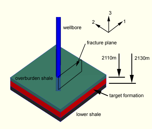
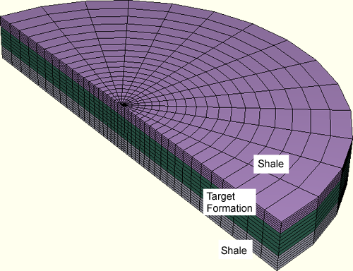
The domain of the problem considered in this example is a 50 m (1969 in) thick circular slice of oil-bearing rock with the well-bore hole modeled. The domain has a diameter of 400 m (15,748 in). Three sections of rock are considered: a region where production oil recovery is targeted, and two surrounding regions of shale. The domain is shown in Figure 9.1.5–1.
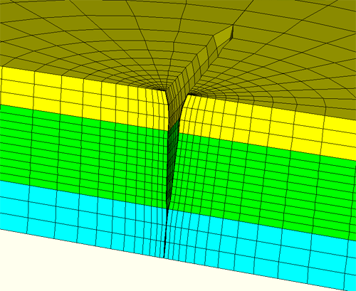
Due to symmetry only a half of the domain is modeled. Figure 9.1.5–2 shows the finite element model. The rock is modeled with C3D8RP elements, and the bore hole casing is modeled with M3D4 elements.
The unopened fracture is modeled along the entire height of the model domain. Cohesive elements (COH3D8P) are used to model a vertical fracture surface.
A linear Drucker-Prager model with hardening is chosen for the rock, while the casing is linear elastic.
The fracture model consists of the mechanical behavior of the fracture itself and the behavior of the fluid that enters and leaks through the fracture surfaces.
The elastic properties of the bonded interface are defined using a traction-separation description, with stiffness values of ![]() =
=![]() =
=![]() = 8.5 × 10⁴ MPa. The quadratic traction-interaction failure criterion is chosen for damage initiation in the cohesive elements; and a mixed-mode, energy-based damage evolution law is used for damage propagation. The relevant material data are as follows:
= 8.5 × 10⁴ MPa. The quadratic traction-interaction failure criterion is chosen for damage initiation in the cohesive elements; and a mixed-mode, energy-based damage evolution law is used for damage propagation. The relevant material data are as follows: ![]() =
= ![]() = 0.32 KPa,
= 0.32 KPa, ![]() =
= ![]() =
=![]() = 28 N/mm, and
= 28 N/mm, and ![]() = 2.284.
= 2.284.
Tangential and normal flow are both modeled in the fracture zone cohesive elements. The following parameters are specified:
Gap flow is specified as Newtonian with a viscosity of 1 × 10⁻⁶ kPaS (1 centepoise), roughly the viscosity of water.
Fluid leakoff is specified as 5.879 × 10⁻¹⁰ m3/(kPa s) for the early stages. In the final stage, when the polymer is dissolved, the fluid leakoff coefficient is increased to 1 × 10⁻³ m3/(kPa s). This step-dependent fluid leakoff coefficient is set in user subroutine UFLUIDLEAKOFF.
An initial geostatic stress field is defined using the user subroutines SIGINI and UPOREP. A depth varying initial void ratio is specified using user subroutine VOIDRI. Gravity loading is specified; and an orthotropic overburden stress state is imposed, with the maximum principle stress in the formation aligned orthogonal to the cohesive element fracture plane.
The analysis consists of four steps:
A geostatic step is performed where equilibrium is achieved after applying the initial pore pressure to the formation and the initial in-situ stresses. The bottom hole shut-in pressure is applied as a traction to the well-bore face.
The next step represents the hydraulic fracture stage where the main volume of fluid is being injected into the well. Flow at a rate of 2.4 m3 (15 barrels) per minute is injected along a targeted 8 m extent in the target formation in the model, and the cohesive elements adjacent to the well bore along this length are defined as initially open to permit entry of fluid. The duration of this stage is 20 minutes.
Following the hydraulic fracture, another transient soils consolidation analysis is conducted. The injection into the well is terminated, and the built-up pore pressure in the fracture is allowed to bleed off into the formation. An additional boundary condition is applied at this stage, fixing the fracture surface open to simulate the behavior of the proppant material that was injected into the fracture.
In the final step a drawdown pressure of 20 kPa is applied to the well-bore nodes of the fracture cohesive elements. This step ends after 100 days of production or when steady-state conditions prevail, defined as pore pressure transients below 0.05 kPa/sec in the model.
The flow injected during Step 2, the pumping stage, initiated and grew a crack extending outward from the well bore. Figure 9.1.5–3 shows the resulting geometry of the fracture at the end of the 20 minute pumping period. These results show that a fracture initiated within the target formation zone tends to avoid the lower shale region, where the compressive stresses are higher, but does infiltrate the upper shale region, where it can decrease well yields.
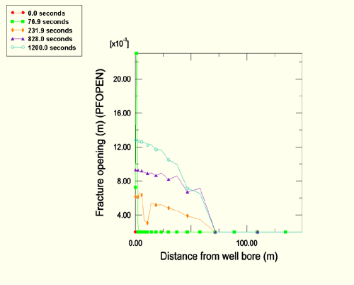
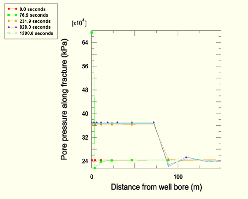
Figure 9.1.5–4 shows the fracture opening profile at various times during the pumping stage; the final profile, shown at 1200 s, is then fixed in the subsequent steps, holding the fracture open with the proppant material. Figure 9.1.5–5 shows a similar history of the pore pressure across the fracture face and indicates that the pore flow has stabilized.
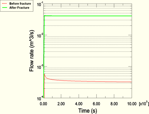
Figure 9.1.5–6 shows the resulting well-bore yield following the hydraulic fracture process. This is compared to an equivalent model where the hydraulic fracturing did not occur. In this simple example the hydraulically fractured well bore shows a marked improvement, with a flow rate more than 100 times the unfractured configuration.