Product: ABAQUS/Standard
This example simulates the settlement of soil near an oil well. It is assumed that the oil in question is too thick for normal pumping. Therefore, steam is injected in the soil in the vicinity of the well to increase the temperature and decrease the oil's viscosity. As a result creep becomes an important component of the soil inelastic deformation and in the prediction of the effects of the oil pumping. Five years of oil pumping are simulated. This coupled displacement/diffusion analysis illustrates the use of ABAQUS to solve problems involving fluid flow through a saturated porous medium, inelastic material properties with time-dependent creep behavior, and thermal loading. No experimental data exist to compare with the numerical results of this example.
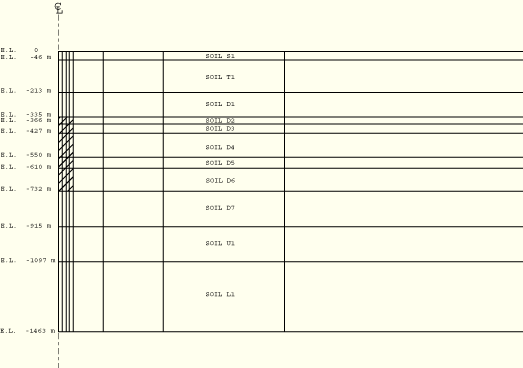
The example considers an axisymmetric model of an oil well and the surrounding soil, as shown in Figure 9.1.3–1. The radius of the well is 81 m (265 ft), and the well extends from a depth of 335 m (1100 ft) to 732 m (2500 ft). A depth of 1463 m (4800 ft) is modeled with 11 different soil layers. Reduced-integration axisymmetric elements with pore pressure, CAX8RP, are used to model the soil in the vicinity of the well. The far-field region is modeled with axisymmetric infinite elements, CINAX5R, to provide lateral stiffness. Reduced integration is almost always recommended when second-order elements are used, because it usually gives more accurate results and is less expensive than full integration. A coarse mesh is selected for the illustrative purpose of this example. No mesh convergence study has been performed.
Soil layers designated by S1, T1, U1, and L1 are modeled using the Drucker-Prager plasticity model and are specified on the *DRUCKER PRAGER option. Both the elastic and inelastic material properties are tabulated in Table 9.1.3–1. The linear form of the Drucker-Prager model with no intermediate principal stress effect (![]() 1.0) is used. The model assumes nonassociated flow; consequently, the material stiffness matrix is not symmetric. The use of UNSYMM=YES on the *STEP option improves the convergence of the nonlinear solution significantly. The hardening/softening behavior is specified by the *DRUCKER PRAGER HARDENING option, and the data are listed in Table 9.1.3–1. No creep data are provided for these layers since these are far removed from the loading. These layers are assumed to be saturated with water. A high permeability is assumed for the two top soil layers S1 and T1, while a low permeability is assigned to layers U1 and L1.
1.0) is used. The model assumes nonassociated flow; consequently, the material stiffness matrix is not symmetric. The use of UNSYMM=YES on the *STEP option improves the convergence of the nonlinear solution significantly. The hardening/softening behavior is specified by the *DRUCKER PRAGER HARDENING option, and the data are listed in Table 9.1.3–1. No creep data are provided for these layers since these are far removed from the loading. These layers are assumed to be saturated with water. A high permeability is assumed for the two top soil layers S1 and T1, while a low permeability is assigned to layers U1 and L1.
Layers D1 through D7 are modeled with the modified Drucker-Prager Cap plasticity model. The material property data are tabulated in Table 9.1.3–2 and are specified by the *CAP PLASTICITY option. As required by the creep model, no intermediate principal stress effect is included (i.e., ![]() 1.0), and no transition region on the yield surface is defined (i.e.,
1.0), and no transition region on the yield surface is defined (i.e., ![]() 0.0). The material's volumetric strain-driven hardening/softening behavior is specified with the *CAP HARDENING option, and the data are listed in Table 9.1.3–2. The initial cap yield surface position,
0.0). The material's volumetric strain-driven hardening/softening behavior is specified with the *CAP HARDENING option, and the data are listed in Table 9.1.3–2. The initial cap yield surface position, ![]() , is set to 0.02. ABAQUS automatically adjusts the position of the cap yield surface if the stress lies outside the cap surface. Consolidation creep is modeled with a Singh-Mitchell type creep model. The creep material data are specified with the *CAP CREEP option and are dependent on temperature. The following creep data are specified:
, is set to 0.02. ABAQUS automatically adjusts the position of the cap yield surface if the stress lies outside the cap surface. Consolidation creep is modeled with a Singh-Mitchell type creep model. The creep material data are specified with the *CAP CREEP option and are dependent on temperature. The following creep data are specified:
| A=2.2E–7 1/day, |
| A=3.5E–4 1/day, |
A uniform thermal expansion coefficient of 5.76E–6 1/°C (3.2E–6 1/°F) and a constant weight density 1.0 metric ton/m3 (64.6 lbs/ft3) are assumed for all layers.
For a coupled diffusion/displacement analysis care must be taken when choosing the units of the problem. The coupled equations may be numerically ill-conditioned if the choice of the units is such that the numbers generated by the equations of the two different fields differ by many orders of magnitude. The units chosen for this example are inches, pounds, and days.
An initial geostatic stress field is defined through the *INITIAL CONDITIONS option and is based on the soil weight density integrated over the depth. A coefficient of lateral stress of 0.85 is assumed. An initial void ratio of 1.5 is used throughout all soil layers with an initial uniform temperature field of 10°C (50°F).
The problem is run in five steps. The first step of the analysis is a *GEOSTATIC step to equilibrate geostatic loading of the finite element model. This step also establishes the initial distribution of pore pressure. Since gravity loading is defined with distributed load type BZ and not with gravity load type GRAV, the pore fluid pressure reported by ABAQUS is defined as the pore pressure in excess of the hydrostatic pressure required to support the weight of pore fluid above the elevation of the material point.
The second step is a *SOILS, CONSOLIDATION step to equilibrate any creep effects induced from the initial geostatic loading step. The choice of the initial time step is important in a consolidation analysis. Because of the coupling of spatial and temporal scales, no useful information is provided by solutions generated with time steps that are smaller than the mesh and material-dependent characteristic time. Time steps that are very much smaller than this characteristic time provide spurious oscillatory results. For further discussion on calculating the minimum time step, refer to “Coupled pore fluid diffusion and stress analysis,” Section 6.7.1 of the ABAQUS Analysis User's Manual. For this example a minimum initial time step of one day was selected.
The third step of the analysis models the injection of steam into the well region between a depth of 366 m to 732 m (1200 ft to 2400 ft). The region is indicated by the shaded area in Figure 9.1.3–1. The nodes in this region are heated to 100°C (212°F) during a *SOILS, CONSOLIDATION analysis. The NO CREEP parameter is included; therefore, creep effects are not considered. The injection of the steam increases the permeability of the oil and increases the soil creep behavior.
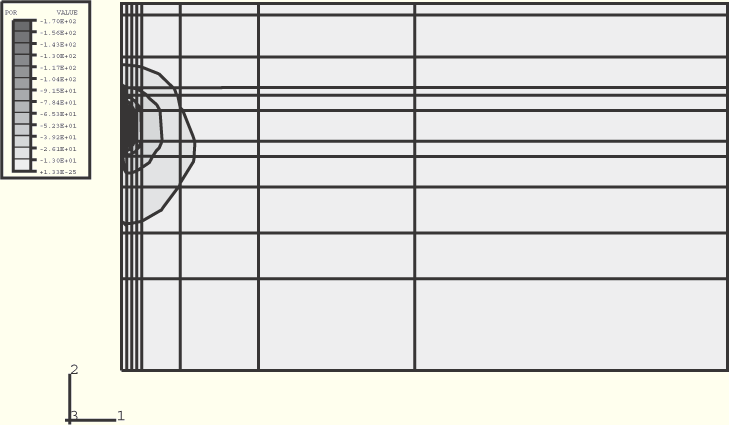
The fourth step simulates the pumping of oil by prescribing an excess pore pressure of –1.2 MPa (–170 psi) at nodes located at the depth of 427 m to 550 m (1400 ft to 1800 ft) below the surface. The pressure produces a pumping rate of approximately 172.5 thousand barrels per day at the end of the fifth year.
The final step consists of a consolidation analysis performed over a five-year period to investigate the settlement that results from pumping and creep effects in the vicinity of the well.
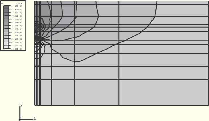
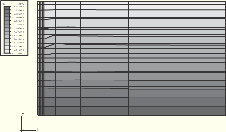
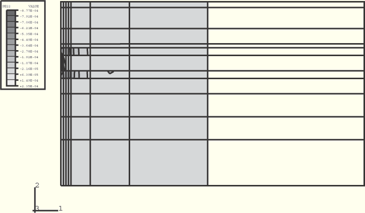
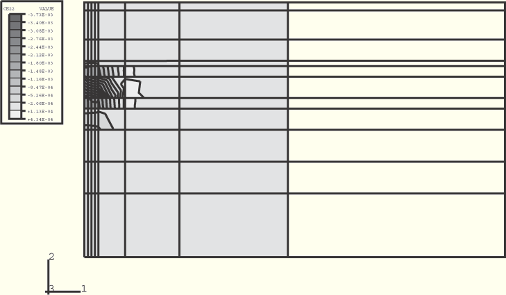
The two initial steps show negligible deformations, indicating that the model is in geostatic equilibrium. Figure 9.1.3–2 shows a contour plot of the soil settlement resulting from consolidation after the five-year period. A settlement of 0.13 m (0.4 ft) is expected at the surface. A maximum soil dislocation of 0.24 m (0.78 ft) occurs above the pump intake. Figure 9.1.3–3 shows a contour plot of the excess pore pressure. The negative pore pressure represents the suction of the pump. During the five-year period, a total of 313.5 million barrels of oil are pumped (as determined from nodal output variable RVT). Figure 9.1.3–4 through Figure 9.1.3–6 show contour plots of the vertical stress components, plastic strains, and creep strains, respectively. Plastification occurs in soil layers D3 through D5. Significant creep occurs in the area in which steam is injected.
Finite element analysis.
Same as axisymoilwell.inp except that the thermal expansion of the pore fluid is also included.
Table 9.1.3–1 Soil data using Drucker-Prager model.
| Soil layer | Elastic properties | Inelastic properties | Hardening behavior |
|---|---|---|---|
| S1 | 0.075 MPa, 0.0 | ||
| K | 0.083 MPa, 0.058 | ||
| 0.075 MPa, 0.116 | |||
| T1 | 0.48 MPa, 0.0 | ||
| K | 0.62 MPa, 0.058 | ||
| 0.48 MPa., 0.116 | |||
| U1 | 1.97 MPa, 0.0 | ||
| K | 3.17 MPa, 0.0037 | ||
| 2.47 MPa, 0.04 | |||
| L1 | 1.97 MPa, 0.0 | ||
| K | 3.17 MPa, 0.0037 | ||
| 2.47 MPa, 0.04 |
Table 9.1.3–2 Soil data using modified Drucker-Prager cap model.
| Soil layer | Elastic properties | Inelastic properties | Hardening behavior | |
|---|---|---|---|---|
| D1 | d | 2.75 MPa, 0.0 | ||
| K | 4.14 MPa, 0.02 | |||
| R | 5.51 MPa, 0.05 | |||
| 6.20 MPa, 0.09 | ||||
| D2 | d | 1.38 MPa, 0.0 | ||
| K | 4.14 MPa, 0.02 | |||
| R | 6.89 MPa, 0.04 | |||
| 55.1 MPa, 0.1 | ||||
| D3 | d | 1.38 MPa, 0.0 | ||
| K | 3.45 MPa, 0.02 | |||
| R | 13.8 MPa, 0.04 | |||
| 62.0 MPa, 0.06 | ||||
| D4 | d | 1.38 MPa, 0.0 | ||
| K | 5.03 MPa, 0.02 | |||
| R | 6.90 MPa, 0.10 | |||
| 62.0 MPa, 0.3 | ||||
| D5 | d | 2.75 MPa, 0.0 | ||
| K | 4.83 MPa, 0.02 | |||
| R | 5.15 MPa, 0.04 | |||
| 62.0 MPa, 0.08 | ||||
| D6 | d | 2.76 MPa, 0.0 | ||
| K | 4.14 MPa, 0.005 | |||
| R | 7.58 MPa, 0.02 | |||
| 62.0 MPa, 0.05 | ||||
| D7 | d | 3.44 MPa, 0.0 | ||
| K | 4.14 MPa, 0.006 | |||
| R | 7.58 MPa, 0.012 | |||
| 67.6 MPa, 0.03 | ||||