Product: ABAQUS/Standard
Joule heating arises when the energy dissipated by electrical current flowing through a conductor is converted into thermal energy. ABAQUS provides a fully coupled thermal-electrical procedure for analyzing this type of problem.
An overview of the capability is provided in “Coupled thermal-electrical analysis,” Section 6.6.2 of the ABAQUS Analysis User's Manual. This example illustrates the use of the capability to model the heating of an automotive electrical fuse due to a steady 30 A electrical current. Fuses are the primary circuit protection devices in automobiles. They are available in a range of different current ratings and are designed so that when the operating current exceeds the design current for a period of time, heating due to electrical conduction causes the metal conductor to melt and—hence—the circuit to disconnect.
A description of the original problem, as well as experimental measurements, can be found in Wang and Hilali (1995). The experimental data and some of the material properties were refined subsequent to this publication. These properties are used here, and the finite element results are compared with the refined measurements (Hilali, July 1995).
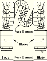
An automotive electrical fuse consists of a metal conductor, such as zinc, embedded within a transparent plastic housing. The plastic housing, which only protects and supports the thin conductor, is not represented in the finite element model. Figure 6.2.1–1 shows front and top sections of the geometry of the conductor. It consists of two 0.76 mm thick blades, with an S-shaped fuse element supported between the blades. The blades fit tightly into standard electrical terminals that are built into the circuit and provide the connection between the electrical circuit and the fuse element. The fuse element is usually much thinner than the fuse blades (in this case 0.28 mm thick) and is designed to melt when the operating current exceeds the design current for a period of time. The fuse blades are 8 mm wide and 30.4 mm long. The fuse element is approximately 3.6 mm wide.
The model is discretized (see Figure 6.2.1–1) with 8-node first-order brick elements (element type DC3D8E), using one element through the thickness. Two 6-node triangular prism elements (element type DC3D6E) are used to fill regions where the geometry precludes the use of brick elements. For comparison refined mesh input files are also included.
The electrical conductivity of zinc varies linearly between 16.75 × 10³ ![]() mm at 20°C and 12.92 × 10³
mm at 20°C and 12.92 × 10³![]() mm at 100°C. The thermal conductivity varies linearly between 0.1120 W/mm°C at 20°C and 0.1103 W/mm°C at 100°C. The density is 7.14 × 10⁻⁶ kg/mm3, and the specific heat is 388.9 J/kg°C. The *JOULE HEAT FRACTION option is used to specify the amount of electrical energy that is converted into thermal energy. We assume that all electrical energy is converted into thermal energy.
mm at 100°C. The thermal conductivity varies linearly between 0.1120 W/mm°C at 20°C and 0.1103 W/mm°C at 100°C. The density is 7.14 × 10⁻⁶ kg/mm3, and the specific heat is 388.9 J/kg°C. The *JOULE HEAT FRACTION option is used to specify the amount of electrical energy that is converted into thermal energy. We assume that all electrical energy is converted into thermal energy.
The analysis is done in two steps. In the first step heating of the conductor due to current flow is considered. Once steady-state conditions are reached, the current is switched off and the fuse is allowed to cooldown to the ambient temperature in a second step. During the first part of the analysis, the coupled thermal-electrical equations are solved for both temperature and electrical potential at the nodes using the *COUPLED THERMAL-ELECTRICAL procedure. In the subsequent cooldown period, since there is no longer any electric current in the fuse, an uncoupled *HEAT TRANSFER analysis (“Uncoupled heat transfer analysis,” Section 6.5.2 of the ABAQUS Analysis User's Manual) is performed. Input files illustrating both steady-state and transient analyses are provided. Steady-state analysis is obtained by specifying the STEADY STATE parameter on the *COUPLED THERMAL-ELECTRICAL procedure. No data lines are required. Transient analysis is available by omitting the STEADY STATE parameter. In this analysis the DELTMX parameter is set to 20°C so that automatic time incrementation is used. The END parameter is set to SS so that the analysis terminates when steady-state conditions are reached. Steady state is defined here as the point at which the temperature rate change is less than 0.1°C/s. This condition is defined on the data line following the *COUPLED THERMAL-ELECTRICAL option. We specify a total analysis time of 100 s, with an initial time step size of 0.1 s.
The electrical loading is a steady 30 A current. This is applied as a concentrated current on each of the nodes on the bottom edge of the left-hand-side terminal. The *CECURRENT option is used for this purpose. The *SECTION FILE option is used to output the total current and the total heat flux in a section defined through the fuse element. The electrical potential (degree of freedom 9) is constrained at the bottom edge of the right-hand-side blade by using a *BOUNDARY option (“Boundary conditions,” Section 27.3.1 of the ABAQUS Analysis User's Manual). This option is also used to keep the bottom edges of the fuse blades at sink temperatures (degree of freedom 11) of 29.4°C and 30.2°C, respectively.
It is assumed that the exposed metal surfaces lose heat through convection to an ambient temperature of ![]() 23.3°C. Heat loss from the thin edges is ignored. The film coefficient varies with temperature according to the empirical relation
23.3°C. Heat loss from the thin edges is ignored. The film coefficient varies with temperature according to the empirical relation
![]()
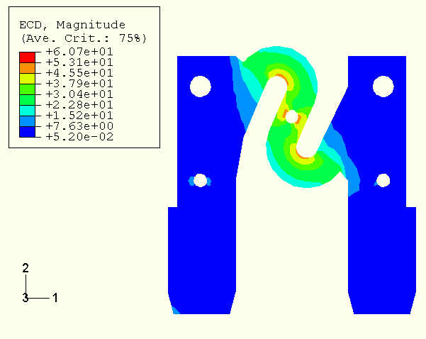
Figure 6.2.1–2 shows a contour plot of the magnitude of the electrical current density vector at steady-state conditions. Since the dissipated electrical energy—and, hence, the thermal energy—is a function of current density, this figure represents contours of the heat generated. The figure indicates that most of the heat is generated near the inside curves of the S-shaped fuse element and near the center hole. The dissipated energy in the fuse blades is negligible compared to that in the fuse element.
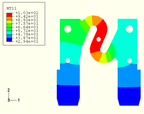
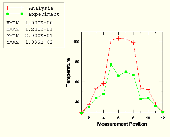
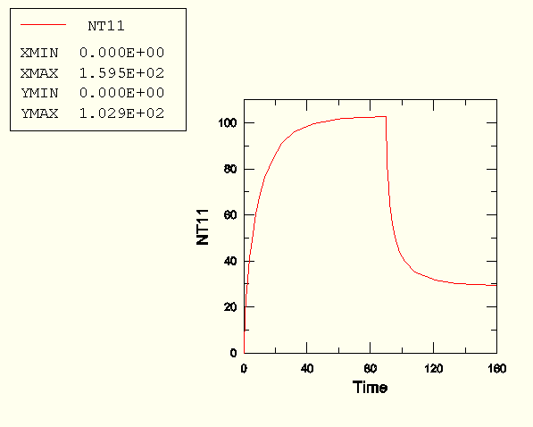
Figure 6.2.1–3 shows a contour plot of the temperature distribution at the end of the first analysis step. The maximum temperature is reached near the center of the S-shaped fuse element. This area is expected to fail first when the operating current exceeds the design current. Figure 6.2.1–4 compares the temperatures at the measuring positions (defined in Figure 6.2.1–1) with the experimental measurements (Hilali, July 1995). While the results show some discrepancies between the experiment and analysis, it is clear that the analysis is sufficiently representative to provide a useful basis for studying such systems. Figure 6.2.1–5 shows the variation of temperature at measuring position 6 during the heating and subsequent cooldown periods.
The results discussed above are for the coarse mesh model. The refined mesh models yield slightly different results from the coarse ones. The maximum difference in the magnitude of the electrical current density vector for the steady-state analysis is approximately 11.4%.
Mr. Hilali and Dr. Wang of Delphi Packard Electric Systems supplied the geometry of the fuse, the material properties, and the experimental results. Delphi Packard assumes no responsibility for the accuracy of the analysis method or data contained in the analysis.
Steady-state analysis.
Transient analysis.
Nodal coordinates for the model.
Element definitions.
Identical to thermelectautofuse_steadystate.inp, except that it uses the *CONTROLS option for control of convergence criteria.
Refined mesh model for the steady-state analysis.
Refined mesh model for the transient analysis.
Hilali, S. Y., Private communication, July 1995.
Hilali, S. Y., and B. -J. Wang, “ABAQUS Thermal Modeling for Electrical Assemblies,” 1995 ABAQUS Users' Conference, Paris, May 1995, pp. 441–457.
Wang, B. -J., and S. Y. Hilali, “Electrical-Thermal Modeling Using ABAQUS,” 1995 ABAQUS Users' Conference, Paris, May 1995, pp. 771–785.