Product: ABAQUS/Standard
This example illustrates the use of the parallel Lanczos eigensolver for modal analysis of a structure. The focus of this example is the usage of the parallel Lanczos eigensolver in conjunction with the different methods of interval splitting that can be applied. In addition, the performance of the parallel Lanczos solver as the number of modes is increased is demonstrated.
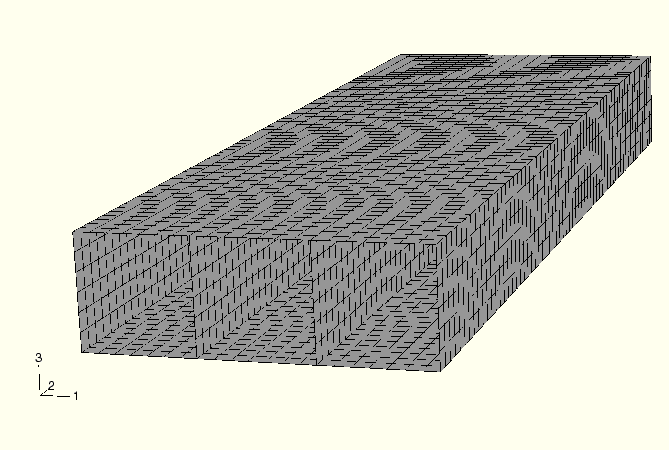
The model used for this study is a relatively simple structure consisting of two flat plates with four stiffeners modeled with S4R elements, as shown in Figure 2.2.4–1. The input files are parametrized such that the number of nodes between stiffeners can be adjusted easily to test the performance of the parallel Lanczos eigensolver as the number of modes or degrees of freedom is changed. The problem consists of finding a specified number of modes using the available splitting strategies. The number of parallel Lanczos frequency intervals (equal to the number of CPUs for all the models shown here) is then increased to study the performance characteristics. The material is elastic, with a Young's modulus of 200 GPa, a Poisson's ratio of 0.3, and a density of 7800 kg/m3. The boundary conditions consist of fixing the right and left edges of the lower plate (parallel to the 3-direction).
The following models are used:
Default splitting strategy. The splitting strategy is chosen by ABAQUS such that the supplied frequency range is split equally among all intervals.
User-specified interval boundaries chosen in all cases such that the same number of eigenvalues is found on each frequency interval.
Biased splitting strategy where the bias parameter, ![]() , is set equal to 2.2.
, is set equal to 2.2.
The models illustrate the use of the parallel Lanczos solver and assume a considerable amount of a priori knowledge about the distribution of the eigenvalues (obtained, for example, by an initial run with *FREQUENCY, NUMBER INTERVAL=1). Even for the default splitting strategy, it is important that the lower and upper frequency bounds, which must both be provided for all parallel Lanczos runs if the number of frequency intervals is greater than 1, be chosen to contain the desired number of eigenmodes. For the user-specified interval boundary models, the boundaries are chosen from the data obtained from the single interval run by selecting the boundaries to partition the overall frequency interval such that the same number of eigenvalues is found on each parallel interval.
To demonstrate the use of the different splitting strategies available for the parallel Lanczos solver and their influence on performance, wallclock timing data are collected for the models described above run on a high-end engineering workstation. A relatively small problem with 24,576 equations and a maximum of 2000 modes extracted is created by setting the number of nodes in the 3-direction to 7 (nnz = 7 in the parametrized input file). For the default and biased splitting analyses, the number of intervals is controlled by specifying NUMBER INTERVAL=4 in the input file and then specifying the number of CPUs to equal the desired number of frequency intervals for a given analysis (this is possible since ABAQUS internally adjusts the number of frequency intervals as described above).
The model is run with NUMBER INTERVAL set equal to 1, 2, and 3 and with 200, 400, 1000, and 2000 modes extracted. In all cases the upper and lower frequencies set on the *FREQUENCY data line are chosen to include exactly the desired number of modes. The wallclock times represent the total run time for the analysis with no output requests (all default output is turned off). Adding nodal output requests adds approximately 5% to the single interval run times, and element output requests will increase the run time by a larger amount. The resulting wallclock times for the default and user-defined splitting are summarized in Table 2.2.4–1. It is clear that there can be a quite substantial benefit to manually entering the frequency interval boundaries, particularly when a large number of modes is extracted. The model where 1000 modes are extracted is run with BIAS=2.2, and the resulting run time is 313 seconds with three intervals. This is comparable to the runs with the user-defined interval boundaries.
200 modes extracted using the default splitting strategy.
400 modes extracted using the default splitting strategy.
1000 modes extracted using the default splitting strategy.
2000 modes extracted using the default splitting strategy.
200 modes extracted with the user-defined splitting strategy on two intervals.
200 modes extracted with the user-defined splitting strategy on three intervals.
400 modes extracted with the user-defined splitting strategy on two intervals.
400 modes extracted with the user-defined splitting strategy on three intervals.
1000 modes extracted with the user-defined splitting strategy on two intervals.
1000 modes extracted with the user-defined splitting strategy on three intervals.
2000 modes extracted with the user-defined splitting strategy on two intervals.
2000 modes extracted with the user-defined splitting strategy on three intervals.
1000 modes extracted with biased splitting on three intervals.