Product: ABAQUS/Standard
This example demonstrates the use of adaptive meshing and adaptive mesh constraints in ABAQUS/Standard to model the large-scale erosion of material such as sand production in an oil well during oil extraction occurring at external surfaces according to local solution-dependent criteria. In ABAQUS/Standard the erosion of material at the external surface is modeled by declaring the surface to be part of an adaptive mesh domain and by prescribing surface mesh motions that recede into the material. ABAQUS/Standard will then remesh the adaptive mesh domain using the same mesh topology but the new location of the surface. All the material point and node point quantities will be advected to their new locations.
The process of optimizing the production value of an oil well is complex but can be simplified as a balance between the oil recovery rate (as measured by the volumetric flow rate of oil), the sustainability of the recovery (as measured by the amount of oil ultimately recovered), and the cost of operating the well. In practice, achieving this balance requires consideration of the erosion of rock in the wellbore, a phenomenon that occurs when oil is extracted under a sufficiently high pressure gradient. This erosion phenomenon is generally referred to as “sand production.” Depending on the flow velocities the sand may accumulate in the well, affecting the sustainability of recovery, or it may get carried to the surface along with the oil. The sand in the oil causes erosion in the piping system and its components such as chokes and pipe bends, increasing the costs of operating the well. Excessive sand production is, therefore, undesirable and will limit oil recovery rates. A typical measure of these limits on recovery rates is the so-called “sandfree rate.” A sandfree rate might be based on direct damage caused by sand production or might be based on the cost of sand management systems that limit the damage of the sand. The former measure is called the maximum sandfree rate, or MSR. The latter measure is called the acceptable sandfree rate, or ASR. The ASR concept has become possible with the availability of many commercial sand management systems as well as new designs of piping components. The ASR concept has also engendered a need for predicting the sand production rates to properly choose and size the sand management systems and piping components. In this example we focus on measures that can be obtained from ABAQUS to predict these rates.
The geometry of an oil well has two main components. The first is the wellbore drilled through the rock. The second component is a series of perforation tunnels that project perpendicular to the wellbore axis. These tunnels, which are formed by explosive shape charges, effectively increase the surface area of the bore hole for oil extraction. The perforation tunnels are typically arranged to fan out in a helical fashion around the bore hole, uniformly offset in both vertical spacing and azimuthal angle.
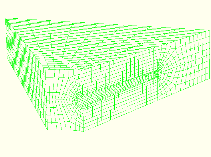
The domain of the problem considered in this example is a 203 mm (8 in) thick circular slice of oil-bearing rock with both the wellbore hole and perforation tunnels modeled. The domain has a diameter of 1.02 m (400 in). The perforation tunnels emanate radially from the bore hole and are spaced 90° apart. Each perforation tunnel is 43.2 mm (1.7 in) diameter and 508 mm (20 in) long. The bore hole has a radius of 158.8 mm (6.25 in). Due to symmetry only a quarter of the domain that contains one perforation tunnel is modeled. Figure 1.1.21–1 shows the finite element model. The rock is modeled with C3D8P elements, and the bore hole casing is modeled with M3D4 elements. A linear Drucker-Prager model with hardening is chosen for the rock, while the casing is linear elastic.
The analysis consists of five steps. First, a geostatic step is performed where equilibrium is achieved after applying the initial pore pressure, the initial stress, and the distributed load representing the soil above the perforation tunnel. The second step represents the drilling operation where the elements representing the bore hole and the perforation tunnel are removed using the element removal capability in ABAQUS (see “Element and contact pair removal and reactivation,” Section 11.2.1 of the ABAQUS Analysis User's Manual). In the third step the boundary conditions are changed to apply the pore pressure on the face of the perforation tunnel. In the fourth step a steady-state soils analysis is carried out in which the pore pressure on the perforation tunnel surface is reduced to the desired drawdown pressure of interest. The fifth step consists of a soils consolidation analysis for four days during which the erosion occurs.
There are two main sources of eroded material in a perforation tunnel. One of the sources is volumetric and is due to the material that is broken up due to high stresses and transported by the fluid through the pores. The other source is surface based and is due to the material that is broken up by the hydrodynamic action of the flow on the surface. Depending on the properties of the oil-bearing strata and the flow velocities, one or the other may be the dominant source of eroded material. Development of equations describing the erosion in a perforation tunnel is an active research field. In this example we consider surface erosion only but choose a form for the erosion equation that has dependencies that are similar to those used by Papamichos and Stavropoulou for volumetric erosion. This approximation is reasonable because high stresses exist only in a very thin layer surrounding the perforation tunnel. The erosion equation is
![]()
Both ![]() and
and ![]() must be determined experimentally. In this example
must be determined experimentally. In this example ![]() ,
, ![]() , and
, and ![]() . We choose
. We choose ![]() as recommended by Papamichos and Stavropoulo. These values are chosen to show visible erosion in a reasonably short analysis time.
as recommended by Papamichos and Stavropoulo. These values are chosen to show visible erosion in a reasonably short analysis time.
The erosion equation describes the velocity of material recession as a local function of solution quantities. ABAQUS/Standard provides functionality through adaptive meshing for imposing this surface velocity, maintaining its progression normal to the surface as the surface moves, and adjusting subsurface nodes to account for large amounts of erosive material loss.
Erosion itself is described through a spatial adaptive mesh constraint, which is applied to all the nodes on the surface of the perforation tunnel. Adaptive mesh constraints can be applied only on adaptive mesh domains; in this example a sufficiently large extent of the finite element mesh, including the perforation tunnel, is declared as the adaptive mesh domain. A cut section of the adaptive mesh domain including the perforation tunnel is shown in Figure 1.1.21–2. Identification of the adaptive mesh domain will result in smoothing of the near-surface mesh that is necessary to enable erosion to progress to arbitrary depths. All the nodes on the boundary of the adaptive mesh domain where it meets the regular mesh must be considered as Lagrangian to respect the adjacent nonadaptive elements.
A velocity adaptive mesh constraint is defined. The generality and solution dependence of the erosion equation are handled by describing the erosion equation in user subroutine UMESHMOTION (see “Defining ALE adaptive mesh domains in ABAQUS/Standard,” Section 12.2.6 of the ABAQUS Analysis User's Manual). User subroutine UMESHMOTION is called at a given node for every mesh smoothing sweep. Mesh velocities computed by the ABAQUS/Standard meshing algorithm for that node are passed into UMESHMOTION, which modifies them to account for the erosion velocities computed at that node. The modified velocities are determined according to the equation for ![]() , where local results are needed for
, where local results are needed for ![]() , n, and
, n, and ![]() . To obtain these values, we request results for output variables PEEQ, VOIDR, and FLVEL respectively, noting that void ratio is related to porosity by
. To obtain these values, we request results for output variables PEEQ, VOIDR, and FLVEL respectively, noting that void ratio is related to porosity by ![]() . Since these output variables are all available at element material points, the utility routine GETVRMAVGATNODE is used to obtain results extrapolated to the surface nodes (see “Obtaining material point information averaged at a node,” Section 2.1.6 of the ABAQUS User Subroutines Reference Manual).
. Since these output variables are all available at element material points, the utility routine GETVRMAVGATNODE is used to obtain results extrapolated to the surface nodes (see “Obtaining material point information averaged at a node,” Section 2.1.6 of the ABAQUS User Subroutines Reference Manual).
Steady state is achieved at the end of the fourth step; therefore, after only one iteration ABAQUS/Standard finds that all the convergence criteria are satisfied and terminates the following consolidation step. The adaptive mesh domain is defined in the fourth step, and adaptive meshing is carried out once at the end of the fourth step. The intention is to perturb the solution to produce some residuals such that a consolidation step could be started from the end of a steady-state step. After the first increment, transients are introduced due to material erosion. The adaptive mesh constraints are applied only in the fifth step when erosion happens.
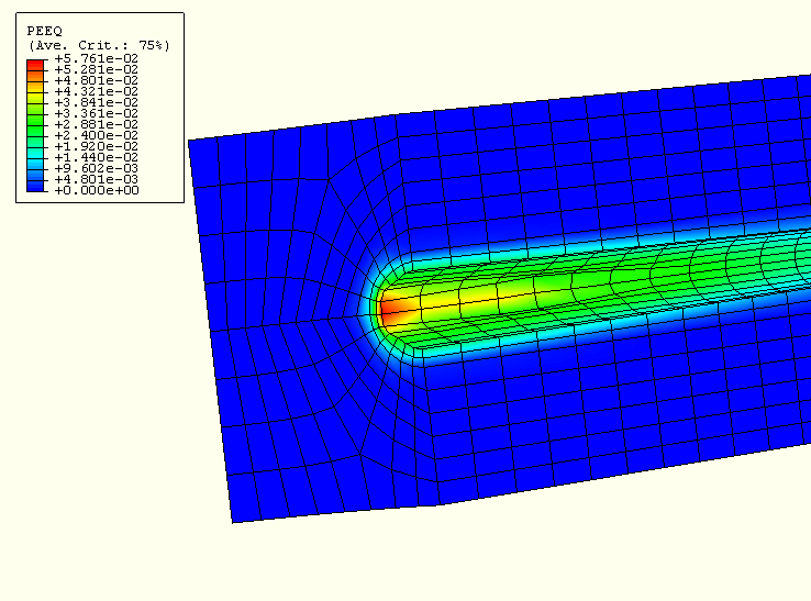
The consolidation analysis in which erosion takes place is run for a time period of four days to observe the initiation of sand production and predict its initial rate. Figure 1.1.21–3 shows the perforation tunnel at the end of four days where it is seen that the largest amount of material is eroded near the junction of the bore hole and perforation tunnel. Further away from the bore hole boundary the amount of erosion progressively decreases. This behavior is expected because there are high strains near the junction of the bore hole and perforation tunnel, and the erosion criterion is active only for values of the equivalent plastic strain above a threshold value.
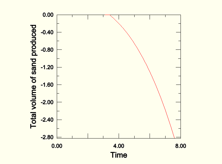
The amount of the volume change due to erosion in an adaptive domain is available using the history output variable VOLC. The actual amount of the solid material eroded depends on the porosity of the rock and is obtained by multiplying VOLC by ![]() . Figure 1.1.21–4 shows the total amount of sand produced in cubic inches over the time period of the consolidation step. As the material is eroded on the surface of the perforation hole tunnel, stresses intensify around the newly eroded boundary leading to an increasingly larger area contributing to the erosion. From Figure 1.1.21–4 it can be concluded that the stresses generated by the drawdown pressure, the fluid velocities, the bore hole and casing geometry, and the initial perforation tunnel geometry are such that this perforation tunnel will produce sand at higher rates as oil recovery continues, although this could be mitigated by further changes to the perforation tunnel caused by the erosion. At a design stage any of these parameters could be modified to limit the sand production rate. Many perforation tunnels emanate from a bore hole, and the total sand production from the bore hole will be the sum total of all the perforation tunnels.
. Figure 1.1.21–4 shows the total amount of sand produced in cubic inches over the time period of the consolidation step. As the material is eroded on the surface of the perforation hole tunnel, stresses intensify around the newly eroded boundary leading to an increasingly larger area contributing to the erosion. From Figure 1.1.21–4 it can be concluded that the stresses generated by the drawdown pressure, the fluid velocities, the bore hole and casing geometry, and the initial perforation tunnel geometry are such that this perforation tunnel will produce sand at higher rates as oil recovery continues, although this could be mitigated by further changes to the perforation tunnel caused by the erosion. At a design stage any of these parameters could be modified to limit the sand production rate. Many perforation tunnels emanate from a bore hole, and the total sand production from the bore hole will be the sum total of all the perforation tunnels.
Model of the oil wellbore hole perforation tunnel.
UMESHMOTION user subroutine.