Product: ABAQUS/Standard
This example illustrates the use of the jointed material model in the context of geotechnical applications. We examine the stability of the excavation of part of a jointed rock mass, leaving a sloped embankment. This problem is chosen mainly as a verification case because it has been studied previously by Barton (1971) and Hoek (1970), who used limit equilibrium methods, and by Zienkiewicz and Pande (1977), who used a finite element model.
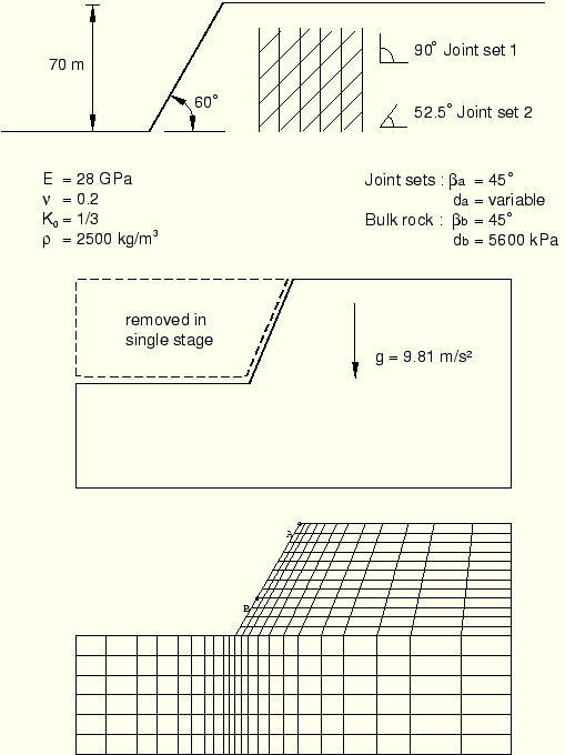
The plane strain model analyzed is shown in Figure 1.1.6–1 together with the excavation geometry and material properties. The rock mass contains two sets of planes of weakness: one vertical set of joints and one set of inclined joints. We begin from a nonzero state of stress. In this problem this consists of a vertical stress that increases linearly with depth to equilibrate the weight of the rock and horizontal stresses caused by tectonic effects: such stress is quite commonly encountered in geotechnical engineering. The active “loading” consists of removal of material to represent the excavation. It is clear that, with a different initial stress state, the response of the system would be different. This illustrates the need of nonlinear analysis in geotechnical applications—the response of a system to external “loading” depends on the state of the system when that loading sequence begins (and, by extension, to the sequence of loading). We can no longer think of superposing load cases, as is done in a linear analysis.
Practical geotechnical excavations involve a sequence of steps, in each of which some part of the material mass is removed. Liners or retaining walls can be inserted during this process. Thus, geotechnical problems require generality in creating and using a finite element model: the model itself, and not just its response, changes with time—parts of the original model disappear, while other components that were not originally present are added. This example is somewhat academic, in that we do not encounter this level of complexity. Instead, following the previous authors' use of the example, we assume that the entire excavation occurs simultaneously.
The jointed material model includes a joint opening/closing capability. When a joint opens, the material is assumed to have no elastic stiffness with respect to direct strain across the joint system. Because of this, and also as a result of the fact that different combinations of joints may be yielding at any one time, the overall convergence of the solution is expected to be nonmonotonic. In such cases the use of *CONTROLS, ANALYSIS=DISCONTINUOUS is generally recommended to prevent premature termination of the equilibrium iteration process because the solution may appear to be diverging.
As the end of the excavation process is approached, the automatic incrementation algorithm reduces the load increment significantly, indicating the onset of failure of the slope. In such analyses it is useful to specify a minimum time step to avoid unproductive iteration.
For the nonassociated flow case UNSYMM=YES is used on the *STEP option. This is essential for obtaining an acceptable rate of convergence since nonassociated flow plasticity has a nonsymmetric stiffness matrix.
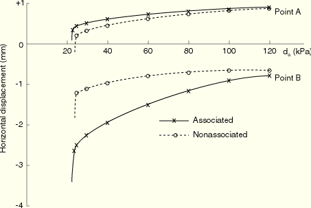
In this problem we examine the effect of joint cohesion on slope collapse through a sequence of solutions with different values of joint cohesion, with all other parameters kept fixed. Figure 1.1.6–2 shows the variation of horizontal displacements as cohesion is reduced at the crest of the slope (point A in Figure 1.1.6–1) and at a point one-third of the way up the slope (point B in Figure 1.1.6–1). This plot suggests that the slope collapses if the cohesion is less than 24 kPa for the case of associated flow or less than 26 kPa for the case of nonassociated flow. These compare well with the value calculated by Barton (26 kPa) using a planar failure assumption in his limit equilibrium calculations. Barton's calculations also include “tension cracking” (akin to joint opening with no tension strength) as we do in our calculation. Hoek calculates a cohesion value of 24 kPa for collapse of the slope. Although he also makes the planar failure assumption, he does not include tension cracking. This is, presumably, the reason why his calculated value is lower than Barton's. Zienkiewicz and Pande assume the joints have a tension strength of one-tenth of the cohesion and calculate the cohesion value necessary for collapse as 23 kPa for associated flow and 25 kPa for nondilatant flow.
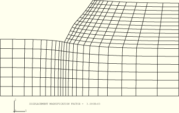
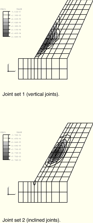
Figure 1.1.6–3 shows the deformed configuration after excavation for the nonassociated flow case and clearly illustrates the manner in which the collapse is expected to occur. Figure 1.1.6–4 shows the magnitude of the frictional slip on each joint system for the nonassociated flow case. A few joints open near the crest of the slope.
Nonassociated flow case problem; cohesion = 30 kPa.
Associated flow case; cohesion = 25 kPa.
Barton, N., “Progressive Failure of Excavated Rock Slopes,” Stability of Rock Slopes, Proceedings of the 13th Symposium on Rock Mechanics, Illinois, pp. 139–170, 1971.
Hoek, E., “Estimating the Stability of Excavated Slopes in Open Cast Mines,” Trans. Inst. Min. and Metal., vol. 79, pp. 109–132, 1970.
Zienkiewicz, O. C., and G. N. Pande, “Time-Dependent Multilaminate Model of Rocks – A Numerical Study of Deformation and Failure of Rock Masses,” International Journal for Numerical and Analytical Methods in Geomechanics, vol. 1, pp. 219–247, 1977.