The plasticity theory for stainless steels, as set forth in nuclear standard NE F9–5T, employs a von-Mises yield surface with kinematic hardening. Ziegler's hardening rule, generalized to the nonisothermal case, is used in ABAQUS.

Normally, when combined isotropic and kinematic hardening is considered, the center of the yield surface is assumed to translate linearly with plastic strain according to a Prager or Ziegler kinematic hardening rule. Incorporation of isotropic hardening into the constitutive formulation then changes the form of the stress-strain relation but leaves the Prager or Ziegler kinematic shift rule for determining the motion of the center of the yield surface intact. In the ORNL plasticity formulation the form of the stress-strain law is left intact (a bilinear representation in one dimension), and modifications to the kinematic shift rule are made to accommodate isotropic hardening.

The Mises yield surface is used:

where is the deviatoric stress and is the kinematic shift (the position of the center of the yield surface in stress space) that is taken to be purely deviatoric, so The quantity is the equivalent uniaxial stress and denotes the distance in stress space from the center of the yield surface to any point on its surface. In the general case this yield surface radius is assumed to depend on the equivalent plastic strain, ; the ORNL defined equivalent creep strain, ; and temperature, .

The model uses associated plastic flow, which means that the plastic strain rate is defined by

where is a scalar that can be identified as the work equivalent plastic strain rate, , defined by This is so because for the Mises yield surface chosen and, thus,

For continued satisfaction of the yield condition (Equation 4.3.8–1) during active plastic straining, the consistency condition is

For the evolution of we use the modified form of Ziegler's hardening rule,

The second term in this equation accounts for isotropic hardening, so when this equation is combined with the consistency condition (Equation 4.3.8–3), the terms containing cancel. This produces a uniaxial stress-strain relation that is bilinear.

The strain rate decomposition during active plastic loading is

(we assume there is no change in the creep strain during active plastic loading). Here is the elastic strain increment, and is the total strain increment.

We use linear elasticity with temperature-dependent moduli, so

where is the elasticity matrix. This gives the rate form where

Combining this with the flow rule (Equation 4.3.8–2) allows the incremental stress-strain relation to be written in the form

Introducing the evolution equation for (Equation 4.3.8–4) into the consistency condition (Equation 4.3.8–3) provides

Projecting Equation 4.3.8–5 onto gives

Combining these two definitions then provides from the total strain rate and temperature change rate as

where and

The incremental stress-strain relationship during active plastic deformation is now obtained directly from Equation 4.3.8–5 as

Reduction of Equation 4.3.8–3 and Equation 4.3.8–4 to one dimension, with at large strain values where , shows that is the slope of the plastic portion of the uniaxial stress versus plastic strain relation.

The incremental stress-strain relation (Equation 4.3.8–6) has the same form as that obtained with pure kinematic hardening. As mentioned previously, this is due to the cancellation of the terms in the expressions for the evolution of and the consistency relation. The bilinear stress-strain law and the translation of the yield surface center are depicted in Figure 4.3.8–1.

In pure kinematic hardening under isothermal conditions the yield center follows the path OCOGOC for two stress reversals under fully reversed strain controlled conditions, while the stress-strain curve follows the path OABCDEFGHAB. In the ORNL theory the translation of the center of the yield surface is governed by Equation 4.3.8–6. The term attains its largest value when and tends to zero under continued cumulative straining as .

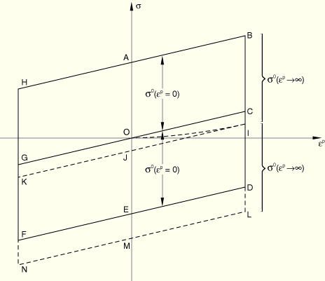
The yield surface center, thus, follows the path OI under monotonic loading. If point I is sufficiently distant from the origin, point O, so that at point I, then as continues to grow under continued stress reversals, the continued growth of is governed by pure kinematic hardening, with . The yield surface center then translates along the path IJKJI. Unlike pure kinematic hardening the ORNL theory, which allows incremental changes in due to cumulative plastic strain, produces a stress-strain curve that is asymmetric about the stress-strain origin.

The expansion of the yield surface is approximated by a step change in the value of . Figure 4.3.8–2 shows the value of appropriate to the virgin (initial) stress-strain curve, , and the value of appropriate to the 10th cycle curve, .

The value of is assumed to undergo a step change according to the relations

These conditions state that a step change in the size of the yield surface occurs when the value of the ORNL equivalent creep strain, , reaches 0.2% or when yielding first occurs after stress reversal. Nuclear standard NE F9–5T recommends that the yield surface center remain fixed during the step change in . In this case the term involving in Equation 4.3.8–6 remains identically equal to zero and the yield surface center translates according to Ziegler's kinematic hardening rule. The nuclear standard recommends that the constant in Equation 4.3.8–6 remain fixed on changing the value of from the virgin to the 10th cycle values. Since is the slope of the stress versus plastic strain in a uniaxial tensile test, this implies that the plastic tangent modulus of the 10th cycle stress-strain curve is the same as the plastic tangent modulus of the virgin stress-strain curve. This requirement is also necessary so that the 10th cycle stress-strain curve under fully reversed strain controlled loading is symmetric about the stress-strain origin.

The flow rule for ORNL creep theory can be written in the form

where is the uniaxial equivalent creep strain rate and is the Mises equivalent stress, The functional dependence of on stress, creep strain, and temperature can be defined either in a user subroutine or by data lines. If the data line option is chosen, ABAQUS assumes that the effective creep strain rate can be written as Under constant stress this gives Elimination of between these equations gives the strain hardening form of the creep law, which is now assumed to be valid even when the stress changes with time.

The ORNL creep theory now replaces the total effective creep strain, , in this equation by an effective creep strain, , determined according to the following algorithm.

At any time during the creep response the equivalent total creep strain used to define the equivalent creep strain rate is defined as the distance from an origin that is either or . indicates at any time which origin is active. If the origin is , we set , while if the origin is , . The quantity defines the distance in total creep strain space between the current origin and the previous origin. The effective creep strain, , is then determined by the following steps:

In addition to the preceding algorithm for the determination of the effective creep strain, , in the strain hardening creep formulation, the ORNL procedures also allow for a translation of the center of the yield surface during creep. Nuclear standard NE F9–5T recommends that the center of the yield surface be shifted during creep according to the relation where the constant being the slope of the uniaxial stress versus plastic strain curve and the current effective yield stress, and is the saturation rate for the kinematic shift caused by creep strain.