For a metal containing a dilute concentration of voids, based on a rigid-plastic upper bound solution for spherically symmetric deformations of a single spherical void, Gurson (1977) proposed a yield condition of the form

where is the deviatoric part of the macroscopic Cauchy stress tensor ; is the Mises stress; is the hydrostatic pressure; is the volume fraction of the voids in the material; and is the yield stress of the fully dense matrix material as a function of , the equivalent plastic strain in the matrix. Tvergaard (1981) introduced the constants , , and (as coefficients of the void volume fraction and pressure terms) to make the predictions of the Gurson model agree with numerical studies of “ordered” voided materials in plane strain tensile fields; one can recover the original Gurson model by setting .

It should be noted that implies that the material is fully dense, and the Gurson yield condition reduces to that of von Mises; implies that the material is fully voided and has no stress carrying capacity. This is illustrated in Figure 4.3.6–1, where the yield surfaces for different levels of porosity are shown in the – plane.

Figure 4.3.6–2 compares the behavior of a porous metal (which has an initial void volume fraction of ) in tension and compression against the perfectly plastic matrix material; the initial yield stress of the porous metal is . In compression the porous material “hardens” due to closing of the voids, and in tension it “softens” due to growth and nucleation of the voids.

The plastic strains are derived from the yield potential; the presence of the first invariant of the stress tensor in the yield condition results in nondeviatoric plastic strains:

where is the nonnegative plastic flow multiplier.

The hardening of the (fully dense) matrix material is described through . The evolution of is assumed to be governed by the equivalent plastic work expression; i.e.,

The change in volume fraction of the voids is due partly to the growth of existing voids and partly to the nucleation of voids. Growth of existing voids is based on the law of conservation of mass and is expressed as

Nucleation of voids can occur due to micro-cracking and/or decohesion of the particle-matrix interface. ABAQUS assumes that the nucleation of new voids is plastic strain controlled (see Chu and Needleman, 1980), so that

where The normal distribution of the nucleation strain has a mean value , a standard deviation , and nucleates voids with volume fraction . The total rate of change of is given as Voids are nucleated only in tension; ABAQUS will not consider the nucleation term at a material point if the stress state is compressive.

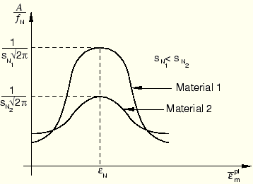
The nucleation function , which is assumed to have a normal distribution, is shown in Figure 4.3.6–3 for different values of the parameter . Figure 4.3.6–4 shows the extent of softening in a uniaxial tension test of a porous material for different values of .

The integration of the elastoplastic equations for the porous plasticity model is carried out using the backward Euler scheme proposed by Aravas (1987). This method is briefly discussed in the following paragraphs; the user can refer to the paper for further details.

During the constitutive calculations in an increment, the stress and state variables are known at time (beginning of the increment). Given a total incremental strain , the stress and state variables need to be updated at (end of the increment) so that they satisfy the yield condition, flow rules, and evolution equation of the state variables. To do this, consider the elasticity equations

where is the elastic predictor and is the linear isotropic elasticity tensor with and being the shear and bulk modulus, respectively, and and being the fourth- and second-order identity tensors, respectively. Also, in the above, the additive decomposition of strain is used to write the total incremental strain as the sum of the elastic and plastic parts. All of the stress and state variables are evaluated at unless indicated otherwise.

The yield condition, the flow rule, and the evolution of the state variables are rewritten as

and where In the above , are the state variables and , respectively. The plastic multiplier is eliminated from the last two equations to give Equation 4.3.6–2 is used in the elasticity Equation 4.3.6–1 to yield and are coaxial; therefore, is determined as Once is known, it is easily seen that consistent determination of the scalars and completes the solution. Therefore, the problem of integrating the pressure-dependent elastoplastic constitutive equations is reduced to solving the following two nonlinear equations for the scalars and : In the above equations , , and are defined by where Equation 4.3.6–8 and Equation 4.3.6–9 are obtained by projecting Equation 4.3.6–4 onto and , respectively, and Equation 4.3.6–10 is an alternate form of Equation 4.3.6–3. Solving the above system of equations for the unknowns and completes the integration algorithm for the porous plasticity model.

Equation 4.3.6–6 and Equation 4.3.6–7 are solved for and using Newton's method; and are updated using Equation 4.3.6–8 and Equation 4.3.6–9; the state variables are updated using Equation 4.3.6–10.

In the implicit finite element method of solving large-deformation problems, the discretized equilibrium equations result in a set of nonlinear equations for the nodal unknowns at the end of the increment. ABAQUS/Standard uses Newton's method to solve these equations, which requires the computation of linearization moduli

To compute (also known as the Jacobian), we start with the elasticity equations (Equation 4.3.6–4), which can be rewritten as where is the deviatoric part of . From the above equation you find that Once again Equation 4.3.6–6 and Equation 4.3.6–7 are used in computing the variations and . After some lengthy algebraic calculations, a set of linear equations is obtained that can be solved for and . These derivatives are substituted into Equation 4.3.6–11 to obtain the linearization moduli. In general this linearization moduli is not symmetric. Further details of the derivation of the Jacobian can be found in Aravas (1987).