Product: ABAQUS/Standard
ABAQUS/Standard includes a library of solid elements whose geometry is initially axisymmetric and that allow for nonlinear analysis in which bending can occur about the plane ![]() in the (
in the (![]() ,
, ![]() ,
, ![]() ) cylindrical coordinate system of the model. The geometric model is defined in the
) cylindrical coordinate system of the model. The geometric model is defined in the ![]() –
–![]() plane only. The displacements are the usual isoparametric interpolations with respect to
plane only. The displacements are the usual isoparametric interpolations with respect to ![]() and
and ![]() , augmented by Fourier expansions with respect to
, augmented by Fourier expansions with respect to ![]() . Since the elements are written for bending about the plane
. Since the elements are written for bending about the plane ![]() only, they cannot be used to model torsion of the structure about the original axis of symmetry. Because the elements are intended for nonlinear applications, the orthogonality properties associated with Fourier modes cannot be used to reduce the problem to a series of smaller, uncoupled, cases, since the stiffness before projection onto the Fourier modes is not necessarily constant. For this reason these elements are significantly more expensive to use than the corresponding axisymmetric elements intended for axisymmetric deformations.
only, they cannot be used to model torsion of the structure about the original axis of symmetry. Because the elements are intended for nonlinear applications, the orthogonality properties associated with Fourier modes cannot be used to reduce the problem to a series of smaller, uncoupled, cases, since the stiffness before projection onto the Fourier modes is not necessarily constant. For this reason these elements are significantly more expensive to use than the corresponding axisymmetric elements intended for axisymmetric deformations.
The coordinate system used with these elements is the cylindrical system (![]() ,
, ![]() ,
, ![]() ), where
), where ![]() measures the distance of a point from the axis of the cylindrical system,
measures the distance of a point from the axis of the cylindrical system, ![]() measures its position along this axis, and
measures its position along this axis, and ![]() measures the angle between the plane containing the point and the axis of the coordinate system and some fixed reference plane that contains the coordinate system axis. The order in which the coordinates and displacements are taken in these elements is based on the convention used in ABAQUS for axisymmetric elements, so that
measures the angle between the plane containing the point and the axis of the coordinate system and some fixed reference plane that contains the coordinate system axis. The order in which the coordinates and displacements are taken in these elements is based on the convention used in ABAQUS for axisymmetric elements, so that ![]() is the second coordinate. This allows these elements to be used in conjunction with other elements in the library that allow only axisymmetric deformation. This order is not the same as that used in three-dimensional elements in ABAQUS in which
is the second coordinate. This allows these elements to be used in conjunction with other elements in the library that allow only axisymmetric deformation. This order is not the same as that used in three-dimensional elements in ABAQUS in which ![]() is the third coordinate, nor is it the order (
is the third coordinate, nor is it the order (![]() ,
, ![]() ,
, ![]() ), usually taken in cylindrical systems.
), usually taken in cylindrical systems.
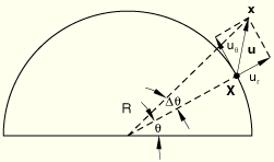
The original geometry of the elements is assumed to be axisymmetric with respect to the axis of the coordinate system and, thus, independent of ![]() . Let
. Let ![]() ,
, ![]() , and
, and ![]() be unit vectors in the radial, axial, and circumferential directions at a point in the undeformed state. The reference position
be unit vectors in the radial, axial, and circumferential directions at a point in the undeformed state. The reference position ![]() of the point can be represented in terms of the original radius
of the point can be represented in terms of the original radius ![]() and the axial position
and the axial position ![]() :
:
![]()
![]()
A general interpolation scheme for ![]() using Fourier terms with respect to
using Fourier terms with respect to ![]() is used:
is used:

We reduce the number of variables in such an element by assuming that bending is allowed only about one plane, ![]() , so that the plane
, so that the plane ![]() ,
, ![]() integer, is a plane of symmetry. The only terms that satisfy this condition are
integer, is a plane of symmetry. The only terms that satisfy this condition are
The ![]() interpolators at the associated positions
interpolators at the associated positions ![]() are taken as
are taken as
![]() :
:
![]()
![]() :
:

![]() :
:
![]() :
:
![]() is the highest-order interpolation offered with respect to
is the highest-order interpolation offered with respect to ![]() in these elements: the elements become significantly more expensive as higher-order interpolation is used; and it is assumed that, because of this, full three-dimensional modeling is less expensive than using these elements with
in these elements: the elements become significantly more expensive as higher-order interpolation is used; and it is assumed that, because of this, full three-dimensional modeling is less expensive than using these elements with ![]() .
.
The integration scheme used in these elements is a product of integration with respect to element coordinates in surfaces that were originally in the ![]() –
–![]() plane and integration with respect to
plane and integration with respect to ![]() . For the former the same scheme is used as in the corresponding purely axisymmetric elements (for example, either full or reduced Gauss integration in the isoparametric quadrilaterals). For integration with respect to
. For the former the same scheme is used as in the corresponding purely axisymmetric elements (for example, either full or reduced Gauss integration in the isoparametric quadrilaterals). For integration with respect to ![]() the trapezoidal rule is used, with the number of integration points set to
the trapezoidal rule is used, with the number of integration points set to ![]() .
.
For a material point in space the deformation gradient ![]() is defined as the gradient of the current position
is defined as the gradient of the current position ![]() with respect to the original position
with respect to the original position ![]() :
:
![]()
![]()
![]()
Since the radial and circumferential base vectors depend on the original circumferential coordinate ![]() :
: ![]() ,
, ![]() , the partial derivatives of these base vectors with respect to
, the partial derivatives of these base vectors with respect to ![]() are nonvanishing:
are nonvanishing:
![]()
To be able to analyze approximately incompressible material behavior, the volume change in the fully integrated 4-node quadrilaterals is assumed to be independent of ![]() and
and ![]() in an
in an ![]() –
–![]() plane. Hence,
plane. Hence, ![]() is modified according to
is modified according to
![]()
![]()

Strain and rotation increments are calculated from the integrated velocity gradient matrix, ![]() , defined as
, defined as
![]()
![]()
The strain increments are approximated as the symmetric part of ![]() :
:
![]()
![]()

The spin increments, ![]() , are approximated as the antisymmetric part of
, are approximated as the antisymmetric part of ![]() , which in matrix form becomes
, which in matrix form becomes
![]()
The formulation of equilibrium (virtual work) requires linearization of the strain-displacement relation in the current state. For fully integrated 4-node elements the volume strain modification provides
![]()
![]()
![]()
![]()
For fully integrated, 4-node quadrilaterals we again use the approximation

The displacements and, hence, the displacement variations, are interpolated in terms of nodal displacement variations with Equation 3.2.9–2. The derivatives of the displacements with respect to ![]() ,
, ![]() , and
, and ![]() are readily obtained from these expressions:
are readily obtained from these expressions:
Since the elements are formulated in terms of Cartesian components of displacements, the equations presented in “Solid element formulation,” Section 3.2.2, apply. For the 4-node quadrilaterals, we can adapt Equation 3.2.2–1 to the averaged volume change formulation, which yields
![]()
![]()
In the 4-node reduced integration element the hourglass modes must be controlled. These modes are similar to the ones in regular axisymmetric elements but have some additional features.
The hourglass pattern can vary along the circumference, which requires application of an hourglass stiffness at multiple points around the circumference.
Hourglassing can also occur in the circumferential direction.
![]()
![]()
![]()
Here ![]() follows from Equation 3.2.9–7, and for
follows from Equation 3.2.9–7, and for ![]() we obtain
we obtain
Similarly, we obtain for the second variation
![]()
For geometrically linear problems equivalent nodal loads due to applied surface pressures and body forces are readily calculated since the geometry is axisymmetric. For geometrically nonlinear problems the treatment of body forces does not change because of the fixed direction of the forces and because the forces are proportional to the volume, which is assumed to change by a negligible amount. However, for surface pressures nonaxisymmetric deformations must be taken into consideration.
The equivalent nodal loads associated with surface pressure ![]() can be obtained by considering the virtual work contribution
can be obtained by considering the virtual work contribution
![]()
![]()
The terms in Equation 3.2.9–8 can be worked out as follows:
Hence, we obtain the virtual work contribution
With use of the interpolation functions we, thus, obtain the equivalent nodal forces:
![]()
![]()
![]()
![]()
![]()
In the case of hydrostatic pressure (![]() dependent on
dependent on ![]() ) some additional terms appear. These terms are readily obtained from the expression
) some additional terms appear. These terms are readily obtained from the expression
With use of the interpolation functions we, thus, obtain the additional load stiffness contributions:
At each material point the displacement components in the three directions (radial, axial, circumferential) are dependent only on the corresponding nodal displacement components. Hence, the mass matrix does not involve any coupling between the radial, axial, and circumferential degrees of freedom, and we can write the mass matrix in the form of three separate expressions:
![]()
![]()
![]()
![]()
The circumferential distribution matrices can be evaluated for various values of the number of terms ![]() in the Fourier series. After some calculations the following results are obtained:
in the Fourier series. After some calculations the following results are obtained:
![]() :
:
![]()
![]() :
:
![]() :
:
![]() :
:
For hybrid and pore pressure elements additional degrees of freedom ![]() are added. In the hybrid elements these degrees of freedom are internal to the element and represent the hydrostatic pressure in the material. In the pore pressure elements the degrees of freedom represent the hydrostatic pressure in the fluid as interpolated from the pressure variables at the external, user-defined nodes. Let the interpolation function for the (hydrostatic or pore) pressure in the
are added. In the hybrid elements these degrees of freedom are internal to the element and represent the hydrostatic pressure in the material. In the pore pressure elements the degrees of freedom represent the hydrostatic pressure in the fluid as interpolated from the pressure variables at the external, user-defined nodes. Let the interpolation function for the (hydrostatic or pore) pressure in the ![]() –
–![]() plane be denoted by
plane be denoted by ![]() . The interpolation functions are the same as for the regular axisymmetric hybrid and pore pressure elements, respectively. Along the circumference, we observe that in the geometrically linear formulation the volumetric strain
. The interpolation functions are the same as for the regular axisymmetric hybrid and pore pressure elements, respectively. Along the circumference, we observe that in the geometrically linear formulation the volumetric strain ![]() only shows cosine dependence:
only shows cosine dependence:
![]()
For a material point in space in the pore pressure element, the pore pressure gradient calculation involves taking derivatives of the pore pressure with respect to the current position ![]() . Again, we do not evaluate the gradient directly but calculate it with respect to the original position
. Again, we do not evaluate the gradient directly but calculate it with respect to the original position ![]() , with the following transformation:
, with the following transformation:
![]()