2.17.1 Stress linearization

Product: ABAQUS/CAE

Stress linearization is the separation of stresses through a section into constant membrane, linear bending, and nonlinearly varying peak stresses. The capability for calculating linearized stresses is available in the Visualization module of ABAQUS/CAE; it is most commonly used for two-dimensional axisymmetric models. See Chapter 33, “Calculating linearized stresses,” of the ABAQUS/CAE User's Manual for detailed information on how to obtain linearized stresses; the computational methods used by ABAQUS are discussed here.

Computing the stress components

Linearized stress components are computed using user-defined sections traversing a finite element model structure. Stress values are extracted at regular intervals along the defined section, and integration is performed numerically using the extracted stress values. Membrane, bending, and peak stress values are computed. These stresses are defined as follows:

Membrane stress

The constant portion of the normal stress such that a pure moment acts on a plane after the membrane stress is subtracted from the total stress.

Bending stress

The variable portion of the normal stress equal to the equivalent linear stress or, where no peak stresses exist, equal to the total stress minus the membrane stress.

Peak stress

The portion of the normal stress that exists after the membrane and bending stresses are subtracted from the total stress.

For the best results, the endpoints of the section should be chosen so that the section is normal to the interior and exterior surfaces of the model. This orientation minimizes problems with shear stresses since they will be approximately zero at the ends of the line (Kroenke, 1973).

Three-dimensional structures

The membrane values of the stress components are computed using the following equation:

where

is the membrane value of stress,
is the thickness of the section,
is the stress along the path, and
is the coordinate along the path.

The linear bending values of the stress components are computed using the following equations:

where

and

are the bending values of the stress at point A and point B (the endpoints of the section; see Figure 2.17.1–1).

Figure 2.17.1–1 Recommended stress paths.

The integration is performed numerically. Assuming the path between point A and point B is divided uniformly into intervals, the integrals are evaluated as follows:

and

where

is the stress at point

along the path.

Axisymmetric structures

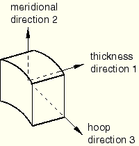
The derivation of the above equations is similar for the axisymmetric case, except for the fact that the neutral axis is shifted radially outward. Separate expressions are obtained for the stresses in the thickness, meridional, and hoop directions. In ABAQUS/CAE these are represented as local directions 1, 2, and 3, respectively (see Figure 2.17.1–2).

Figure 2.17.1–2 Stress directions.

Meridional stress

The meridional stresses are computed using the following relations. The meridional force per unit circumferential length is

where

is the stress in the meridional direction,
is the radius of the point being integrated, and
is the mean circumferential radius.

The meridional membrane stress

is obtained by dividing

through the thickness:

The numerical scheme used to compute the meridional membrane stress is

where

is the meridional stress component at point along the path and
is the radius at point along the path.

To compute the meridional bending stresses, we first need to compute the distance from the center surface to the neutral surface for meridional bending. That distance,

, is equal to

where

is the angle between the thickness direction and the radial direction.

The meridional bending moment per unit circumferential length is defined as

and the moment of inertia for meridional bending is given by

Hence, the meridional bending stresses at the endpoints A and B are obtained with

The numerical scheme used to compute the meridional bending moment is

Hoop stress

The hoop membrane stress is obtained with

where

is the hoop stress and
is the radius of curvature of the midsurface of the section in the meridional plane.

The hoop bending stresses at the endpoints are obtained using the relations

where

is the distance from the center surface to the neutral surface for hoop bending,

is the hoop bending moment per unit meridional length, and

is the moment of inertia for circumferential bending.

The numerical scheme to compute the circumferential membrane stress is

and the bending moment is computed with the summation

Thickness stress

The thickness stress does not transfer any forces or moments. Typically, the stress arises due to applied external pressures and thermal expansion effects, and there is no obvious preferred method for determining “membrane” and “bending” stresses. Hence, we choose the thickness “membrane” stress as the average thickness stress:

We choose the thickness “bending” stress such that the sum of the thickness membrane and bending stresses at the endpoints A and B is equal to the total stress at these points:

and interpolate the bending stress linearly between these values. This is a reasonable assumption, since the thickness surface stresses are determined by the applied pressure and should not have a strong “peak” stress contribution.

Shear stress

The membrane shear stress in the meridional plane is computed in the same way as the meridional membrane stress:

where

is the shear stress along the path.

The shear stress distribution is assumed to be parabolic and equal to zero at the ends. Hence, the bending shear stresses are set to 0.0. The numerical scheme used to compute the membrane shear stress is:

Curvature correction in nonaxisymmetric structures

The equations used when performing stress linearization in axisymmetric structures include the in-plane and out-of-plane radius of curvature of the stress line section. ABAQUS/CAE allows the inclusion of these “curvature correction” terms in the equations for nonaxisymmetric structures when computing the S22, S33, and S12 components. The numerical scheme is identical to that used when performing stress linearization in axisymmetric structures. The user is required to select a coordinate system in which to specify the curvature correction terms. An error will be generated when the -axis of the coordinate system is normal to the stress line.

Computing the local coordinate system

Stress linearization requires the results to be transformed from the global coordinate system to a local coordinate system defined by the stress line.

Axisymmetric case

The computation of the local coordinate system is a trivial procedure when performed for axisymmetric stress linearization. The transformation matrix in this case will be

Three-dimensional case

When performing three-dimensional stress linearization, the local -axis will be defined by the stress line. The local - and -axes are computed by a series of cross-products. This procedure is shown below.