The kinematics of the rolling problem are described in terms of a coordinate frame that moves along with the ground motion of the body. In this moving frame the rigid body rotation is described in a spatial or Eulerian manner and the deformation in a material or Lagrangian manner. It is this kinematic description that converts the steady moving contact field problem into a purely spatially dependent simulation.

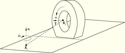
We consider the case shown in Figure 2.7.1–1, where the ground velocity of the body is described in terms of a constant cornering motion.

The body is rotating with a constant angular rolling velocity around a rigid axle at , which in turn rotates with constant angular velocity around the fixed cornering axis through point . Hence, the motion of a particle at time consists of a rigid rolling rotation to position , described by followed by a deformation to point , and a subsequent cornering rotation (or precession) around to position so that where is the cornering rotation given by and is the skew-symmetric matrix associated with the rotation vector . Similarly, is the spinning rotation matrix defined as and is the skew-symmetric matrix associated with the rotation vector . The velocity of the particle then becomes To describe the deformation of the body, we define a map , which gives the position of point at time as a function of its location at time so that It follows that where Noting that , and introducing the circumferential direction , where is the radius of a point on the reference body, the velocity of the reference body can be written as , so that where is the distance-measuring coordinate along the streamline. Using this result, together with , the velocity of the particle can be written as The acceleration is obtained by a second differentiation and some manipulation:

To obtain expressions for the velocity and acceleration in the reference frame tied to the body, we use the transformations

so that we obtain and For steady-state conditions these expressions reduce to and

The first term in the last expression can be identified as the acceleration that gives rise to centrifugal forces resulting from rotation about . Noting that is a measure of velocity, the second term can be identified as the acceleration that gives rise to Coriolis forces. The last term combines the acceleration that gives rise to Coriolis and centrifugal forces resulting from rotation about . When the deformation is uniform along the circumferential direction, this Coriolis effect vanishes so that the acceleration gives rise to centrifugal forces only.

The velocity of the center of the body (which must lie on the axis ) is

since the motions due to rolling and deformation vanish on the axis.

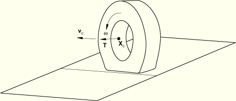
To obtain the expression for straight line motion, as shown in Figure 2.7.1–2, we move far away from the center of the body but keep the same. In that case and, hence, in the limit

which corresponds to straight line rolling.

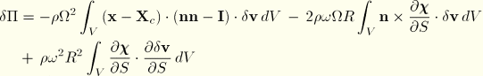
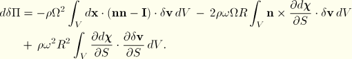
The virtual work contribution from the d'Alembert forces is

Using the divergence theorem, the virtual work contribution becomes and the rate of virtual work becomes For straight line rolling only the last term in each expression needs to be taken into account.

To obtain the contact conditions, we start with the expressions for velocity derived in the previous section. For points on the surface of the deformable body

where is the cornering axis (which must be normal to the rigid surface) and is the cornering angular velocity around . Assuming that the velocity of a point on the foundation (or rigid surface) is , the relative motion becomes where . This equation can be split into normal and tangential components. The rate of penetration is For any point in contact ; hence, which in incremental form reduces to the standard contact condition For steady-state conditions and .

Similarly, the rate of slip is

where are two orthogonal unit vectors tangent to the contact surface so that . For steady-state conditions , so Variations in yield For straight line rolling we can replace by so that we obtain and

To complete the formulation, a relationship between frictional stress and slip velocity must be developed. A Coulomb friction law is provided for steady-state rolling. The law assumes that slip occurs if the frictional stress,

is equal to the critical stress, , where and are shear stresses along , is the friction coefficient, and is the contact pressure. On the other hand, when , no relative motion occurs. The condition of no relative motion is approximated in ABAQUS by stiff viscous behavior where is the tangential slip velocity and is the “stick viscosity,” which follows from the relation The allowable viscous slip velocity is defined as a fraction of the circumferential velocity where is a user-defined slip tolerance.

These expressions contribute to the standard virtual work contribution for slip,

and rate of virtual work for slip,