General contact interactions typically are defined by specifying self-contact for a default, element-based surface defined automatically by ABAQUS/Explicit that includes all bodies in the model. To refine the contact domain, you can include or exclude specific surface pairs. Contact pair interactions are defined by specifying each of the individual surface pairs that can interact with each other.
The definition of surfaces is part of the model data. General contact can be defined as either model or history data; contact pairs are always defined as history data.
Surfaces are created using the *SURFACE option. The TYPE parameter on this option dictates the type of surface created:
The TYPE=ELEMENT parameter (default) on the *SURFACE option creates a surface by specifying the underlying element faces forming the surface.
The TYPE=NODE parameter on the *SURFACE option creates a pure slave surface composed of the specified set of nodes. Nodes on any elements can be part of this node-based surface. For several reasons, including more accurate frictional forces and the ability to use the balanced master-slave approach, it is better to use the *SURFACE option without the parameter TYPE=NODE when possible.
The concepts of master and slave surfaces are discussed later in this chapter.
The TYPE parameter on the *SURFACE option can also be used to specify the specific form of an analytical rigid surface. The different values that the TYPE parameter can take in this case are discussed later in this chapter.
Surfaces on continuum elements
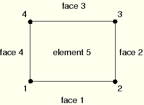
A two-dimensional, first-order continuum element, such as CPE4R, has four faces consisting of the segments defined by nodes 1–2, 2–3, 3–4, and 4–1, respectively, as shown in Figure 6–1. The face identifiers consist of the letter “S” followed by the face number. A surface is defined by specifying the element number and face identifier for all the faces that form the surface.
For example, use the following option block to include face 2 of the element shown in Figure 6–1 in a surface called FLANGE1:*SURFACE, NAME=FLANGE1 5, S2
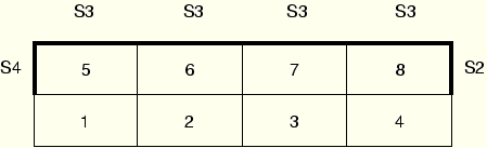
As is the case for many options in ABAQUS, both element numbers and element sets can be used; the use of element sets can make the definition of large surfaces much easier. It is valid to specify both element sets and individual elements in the same *SURFACE option block. For example, the surface TOPSURF consists of the element faces shown in Figure 6–2 and is created as follows:
*ELSET, ELSET=TOP, GENERATE
5, 8
*SURFACE, NAME=TOPSURF
TOP, S3
5, S4
8, S2
ABAQUS can determine the free faces of two- and three-dimensional continuum elements automatically and use them to create a surface. To use this capability, simply include all of the elements whose free faces compose the surface on the data lines of the *SURFACE option. Element sets as well as individual element numbers can be used. ABAQUS will ignore any elements that do not contain free faces. For example, the surface shown in Figure 6–2 could also be defined as follows:
*SURFACE, NAME=TOPSURF
TOP,
While generally not necessary, surfaces on continuum elements also can be defined by a set of nodes. To define a node-based surface, specify node numbers or node sets on the data lines following the *SURFACE, TYPE=NODE option.
Surfaces on shell, membrane, and rigid elements
There are three ways to define surfaces on shell, membrane, and rigid elements: using single-sided surfaces, double-sided surfaces, and node-based surfaces.
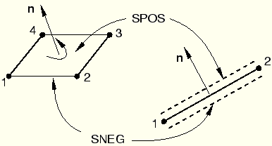
Using single-sided contact surfaces, you select one of the two available faces as a contact surface. The face whose normal points in the direction of the positive element normal is called SPOS, while the face whose normal points in the direction of the negative element normal is called SNEG, as shown in Figure 6–3.
Using the right-hand rule, the nodal ordering of an element defines the positive element normal. By default, the contact surface is the actual element surface, taking into consideration the thickness of the element. When using shell elements, you can instead specify the shell reference surface (the surface defined by the nodes) as the contact surface by neglecting the shell thickness in the contact calculations. The following option block defines surface SURF1 as the surface composed of all the SPOS faces of the elements in element set SHELLS:*SURFACE, NAME=SURF1 SHELLS, SPOS
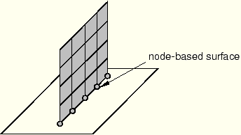
Node-based surfaces can be used to define contact between a set of nodes and a surface. The following option block defines a node-based surface named EDGE, composed of the edge nodes in a node set called NEDGE:
*SURFACE, TYPE=NODE, NAME=EDGE
NEDGE,
This type of surface can be used when defining contact on a shell edge, as shown in Figure 6–4.
Double-sided contact surfaces are more general because both the SPOS and SNEG faces and all free edges are included automatically as part of the contact surface. Contact can occur on either face or on the edges of the elements forming the double-sided surface. For example, a slave node can start on one side of a double-sided surface and then travel around the perimeter to the other side during the course of an analysis. No face identifier is specified when defining double-sided contact because both faces are included automatically. Currently, double-sided surfaces are available only for three-dimensional elements. The general contact algorithm and self-contact in the contact pair algorithm enforce contact on both sides of all shell, membrane, and rigid surface facets, even if they are defined as single-sided. The following option block defines surface SURF2 as the surface composed of both faces of the elements in element set SHELLS:
*SURFACE, NAME=SURF2
SHELLS,
Rigid surfaces
Rigid surfaces are the surfaces of rigid bodies. They can be defined as an analytical shape, or they can be based on the underlying surfaces of elements associated with the rigid body.
Analytical rigid surfaces are created by defining a series of connected lines, arcs, and parabolas. The ANALYTICAL SURFACE parameter on the *RIGID BODY option binds an analytical rigid surface (defined with the TYPE parameter on the *SURFACE option) with a rigid body. The *RIGID BODY option must be defined in the model definition. The TYPE parameter on the *SURFACE option defines the dimensionality of the surface, and it has three possible values:
Use TYPE=SEGMENTS to define a two-dimensional analytical rigid surface.
Use TYPE=CYLINDRICAL to define a three-dimensional analytical rigid surface that is extruded infinitely in the out-of-plane direction.
Use TYPE=REVOLUTION to define a three-dimensional analytical rigid surface of revolution.
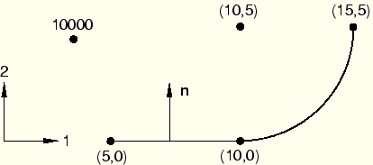
The following is an example input for the two-dimensional analytical rigid surface named SRIGID shown in Figure 6–5:
*SURFACE, TYPE=SEGMENTS, NAME=SRIGID
START, 5.0, 0.0
LINE, 10.0, 0.0
CIRCL, 15.0, 5.0, 10.0, 5.0
where the rigid body is defined previously by
*RIGID BODY, ANALYTICAL SURFACE=SRIGID, REF NODE=10000
Discretized rigid surfaces are based on the underlying elements that make up a rigid body; thus, they can be more geometrically complex than analytical rigid surfaces. Discretized rigid surfaces are defined using the *SURFACE option in exactly the same manner as surfaces on deformable bodies.
Currently, analytical rigid surfaces can be used only with the contact pair algorithm.
You must specify the contact algorithm that will be used to model the interactions between surfaces.
Contact pairs
Define possible contact between two surfaces in an ABAQUS simulation by specifying the surface names on the *CONTACT PAIR option. A surface can appear in any number of contact pairs.
Each contact pair can refer to a surface interaction definition, in much the same way that each element must refer to an element property definition. Use the INTERACTION parameter on the *CONTACT PAIR option to refer to a *SURFACE INTERACTION option, through which the different surface interaction models, such as *FRICTION, can be defined.
The following example specifies that surfaces FLANGE1 and FLANGE2 can interact with each other and assigns a surface interaction model called FRIC to this interaction:
*CONTACT PAIR, INTERACTION=FRIC
FLANGE1, FLANGE2
A surface may contact itself if only one surface is given on the *CONTACT PAIR option; for example,
*CONTACT PAIR, INTERACTION=FRIC
TUBE,
Single-surface contact is somewhat more computationally expensive with the contact pair algorithm than two-surface contact. However, single-surface contact is useful if a surface folds over and contacts itself during the analysis. In such cases it is not possible to identify prior to the analysis which parts of the surface will interact.
General contact
Define a general contact interaction by including the *CONTACT and *CONTACT INCLUSIONS options in your input file. Typically, general contact interactions are defined for a default, all-inclusive surface defined automatically by ABAQUS/Explicit that spans all the bodies in the model. Use the *CONTACT INCLUSIONS and *CONTACT EXCLUSIONS options to refine the contact domain by including or excluding specific surface pairs.
Each general contact definition can refer to a surface interaction definition, in much the same way that each element refers to an element property definition. Use the *CONTACT PROPERTY ASSIGNMENT option to assign a surface interaction model to specified regions of the general contact domain. Use the *SURFACE INTERACTION option to define different surface interaction models, such as *FRICTION.
The following example specifies that all surfaces in the model can interact with each other and assigns a surface interaction model called FRIC to the entire contact domain:
*CONTACT
*CONTACT INCLUSIONS, ALL ELEMENT BASED
*CONTACT PROPERTY ASSIGNMENT
 , , FRIC
In contrast to the contact pair algorithm, this approach does not require explicit definition and pairing of surfaces.
The contact formulation includes the constraint enforcement method, the contact surface weighting, the tracking approach, and the sliding formulation.
Constraint enforcement method
For general contact ABAQUS/Explicit enforces contact constraints using a penalty contact method, which searches for node-into-face and edge-into-edge penetrations in the current configuration. The penalty stiffness that relates the contact force to the penetration distance is chosen automatically by ABAQUS/Explicit so that the effect on the time increment is minimal yet the penetration is not significant. The penalty stiffness can be overridden by specifying a penalty scale factor or a “softened” contact relationship.
For the contact pair algorithm ABAQUS/Explicit uses a kinematic contact formulation by default that achieves precise compliance with the contact conditions using a predictor/corrector method. The increment at first proceeds under the assumption that contact does not occur. If at the end of the increment there is an overclosure, the acceleration is modified to obtain a corrected configuration in which the contact constraints are enforced. The predictor/corrector method used for kinematic contact is discussed in more detail in “Contact formulation for ABAQUS/Explicit contact pairs,” Section 21.4.4 of the ABAQUS Analysis User's Manual; some limitations of this method are discussed in “Common difficulties associated with contact modeling using the contact pair algorithm in ABAQUS/Explicit,” Section 21.4.6 of the ABAQUS Analysis User's Manual.
The normal contact constraint for contact pairs can optionally be enforced with the penalty contact method, which can model some types of contact that the kinematic method cannot. For example, the penalty method allows modeling of contact between two rigid surfaces (except when both surfaces are analytical rigid surfaces). When the penalty contact formulation is used, equal and opposite contact forces with magnitudes equal to the penalty stiffness times the penetration distance are applied to the master and slave nodes at the penetration points. The penalty stiffness is chosen automatically by ABAQUS/Explicit and is similar to that used by the general contact algorithm. A penalty scale factor can also be specified. To select the penalty method for a contact pair analysis, set the MECHANICAL CONSTRAINT parameter to PENALTY on the *CONTACT PAIR option.
Contact surface weighting
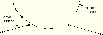
In the pure master-slave approach one of the surfaces is the master surface and the other is the slave surface. As the two bodies come into contact, the penetrations are detected and the contact constraints are applied according to the constraint enforcement method (kinematic or penalty). Pure master-slave weighting (regardless of the constraint enforcement method) will resist only penetrations of slave nodes into master facets. Penetrations of master nodes into the slave surface can go undetected, as shown in Figure 6–6, unless the mesh on the slave surface is adequately refined.
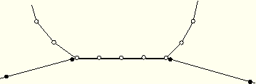
Balanced master-slave contact simply applies the pure master-slave approach twice, reversing the surfaces on the second pass. One set of contact constraints is obtained with surface 1 as the slave, and another set of constraints is obtained with surface 2 as the slave. The acceleration corrections or forces are obtained by taking a weighted average of the two calculations. For kinematic balanced master-slave contact a second correction is made to resolve any remaining penetrations, as described in “Contact formulation for ABAQUS/Explicit contact pairs,” Section 21.4.4 of the ABAQUS Analysis User's Manual. The balanced master-slave contact constraint when kinematic compliance is used is illustrated in Figure 6–7.
The balanced approach minimizes the penetration of the contacting bodies and, thus, provides more accurate results in most cases.The general contact algorithm uses balanced master-slave weighting whenever possible; pure master-slave weighting is used for general contact interactions involving node-based surfaces, which can act only as pure slave surfaces. Use the *CONTACT FORMULATION, TYPE=PURE MASTER-SLAVE to specify pure master-slave weighting for other general contact interactions.
For the contact pair algorithm ABAQUS/Explicit will decide which type of weighting to use for a given contact pair based on the nature of the two surfaces involved and the constraint enforcement method used. The weight of the average can be specified by the user for balanced master-slave contact with the contact pair algorithm using the WEIGHT parameter on the *CONTACT PAIR option. For most element types the default weight is 0.5 so that the same weight is used for each of the acceleration corrections. Setting WEIGHT to 1.0 specifies a pure master-slave relationship with the first surface as the master surface. Conversely, a weight of zero means that the second surface is the master surface.
Tracking approach
Because it is possible for a node on one contact surface to contact any of the facets on the opposite contact surface, ABAQUS/Explicit uses sophisticated search algorithms for tracking the motions of the contact surfaces. While the contact search algorithm is transparent to the user and is rarely a concern, some situations require special consideration and an understanding of the methods. The discussion that follows applies to contact pair interactions. The general contact algorithm uses a somewhat more sophisticated global/local tracking approach that does not require user control.
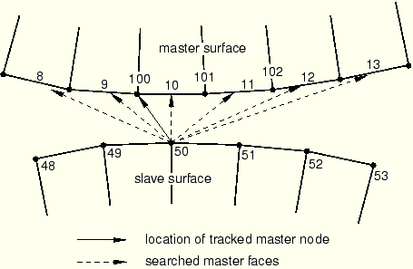
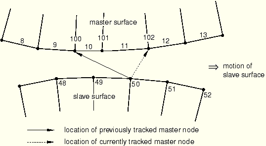
At the beginning of each step an exhaustive, global search is conducted to determine the closest master surface facet for each slave node of each contact pair. This search is aided by a “bucket sort,” but the cost of a global search is relatively high. A global search is performed only every 100 increments by default. Figure 6–8 shows the global search to determine which of all of the facets on the master surface is the closest facet to slave node 50. The search determines that the closest master facet is the face of element 10. Node 100 is determined to be the node on that master facet that is closest to slave node 50; therefore, it is designated as the tracked master surface node. The goal of the global search is to determine the closest master facet and a tracked master surface node for each slave node.
Since the cost of each global search is relatively high, a less expensive local search is performed in most increments. In a local search a given slave node searches only the facets that are attached to the previous tracked master surface node to determine the closest facet. In Figure 6–9 the slave surface of the model shown in Figure 6–8 has moved since the previous increment. (The relative incremental motion shown is much greater than typically occurs in an explicit dynamic analysis because of the small time increments used.) Since the previous tracked master surface node was 100, the nearest master surface facet of those attached to node 100 (facets 9 and 10) is determined.
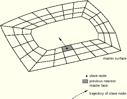
In this case facet 10 is the closest to node 50. The next step is to determine the current tracked master surface node from the nodes attached to facet 10. This time node 101 is the closest node on facet 10 to slave node 50. The local search continues until the tracked master surface node remains the same from one iteration of the search to the next. In this case the tracked master surface node changed from 100 to 101, so the local search continues. Again, the closest master facet is determined from the master facets attached to node 101, in this case facets 10 and 11. Facet 11 is determined to be the closest facet, and node 102 is determined to be the new tracked master surface node. Since node 102 is truly the closest master node to slave node 50, further iteration does not change the tracked master surface node, and the local search ends.Since the time increments are very short, for most situations the contacting bodies move a very small amount from one increment to the next, and the local contact search is adequate to track the motion of the contact surfaces. However, there are certain situations that may cause the local contact search to fail. One such situation, illustrated in Figure 6–10, is a master surface containing a hole.
The shaded element face has been identified as the closest master facet to the slave node belonging to a separate, contacting body. Thus, ABAQUS/Explicit conducts a local search of the master facet and its neighbors for contact in the next increment. If the slave node later displaces across the hole and reaches the other side before another global search is performed, the local search algorithm will still be checking only the shaded facet and its neighbors. Potential contact between the slave node and master facets across the hole will not be recognized in the local contact search. To overcome the problem, ABAQUS/Explicit can be forced to perform a global contact search more often because a global search will recognize contact across the hole. To force the global contact search more often than the default (every 100 increments), set the GLOBTRKINC parameter on the *CONTACT CONTROLS option equal to the desired number of increments between global contact searches. Use caution when using the GLOBTRKINC parameter because frequent global contact searches are computationally expensive.Another option is to allow a single surface to contact itself. For example, the inside of a tube could be defined as a single surface, which contacts itself as the tube is crushed. Due to the generality and complexity of single-surface contact with the contact pair algorithm, a global contact search is performed every few increments, making single-surface contact significantly more expensive than two-surface contact.
Sliding formulation
When defining a contact pair, you must decide whether the magnitude of the relative sliding will be small or finite. The default (and only option for general contact interactions) is the more general finite-sliding formulation. Small sliding is appropriate if the relative motion of the two surfaces is less than a small proportion of the characteristic length of an element face. The small-sliding formulation is selected by including the SMALL SLIDING parameter on the *CONTACT PAIR option. Using the small-sliding formulation when applicable results in a more efficient analysis.
Each contact interaction can refer to a *SURFACE INTERACTION option block that specifies a model for the interaction between the contacting surfaces. There are several contact interaction models available in ABAQUS/Explicit; the default model is frictionless contact with no bonding.
Friction model
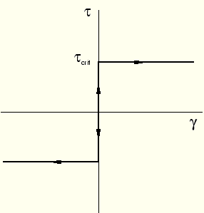
When surfaces are in contact, they usually transmit shear as well as normal forces across their interface. Thus, the analysis may need to take frictional forces, which resist the relative sliding of the surfaces, into account. Coulomb friction is a common friction model used to describe the interaction of contacting surfaces. If the *FRICTION option is used, ABAQUS/Explicit uses a Coulomb friction model to resist relative tangential motion between contacting surfaces. The model characterizes the frictional behavior between the surfaces using a coefficient of friction, ![]() . If the *FRICTION option is not used, the default friction coefficient is zero. The tangential motion is zero until the surface traction reaches a critical shear stress value, which depends on the normal contact pressure, according to the following equation:
. If the *FRICTION option is not used, the default friction coefficient is zero. The tangential motion is zero until the surface traction reaches a critical shear stress value, which depends on the normal contact pressure, according to the following equation:
![]()
The *FRICTION option is a suboption of the *SURFACE INTERACTION option. In the following example, a coefficient of friction of 0.1 is defined with a friction stress limit of 80 MPa:
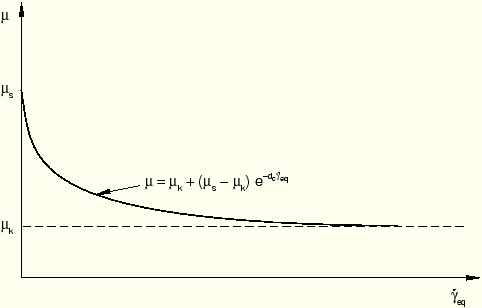
*SURFACE INTERACTION, NAME=INTER
*FRICTION, TAUMAX=80.0E6
0.1,
Often the friction coefficient at the initiation of slipping from a sticking condition is different from the friction coefficient when sliding. The former is typically referred to as the static friction coefficient, and the latter is referred to as the kinetic friction coefficient. In ABAQUS/Explicit an exponential decay law is available to model the transition between static and kinetic friction (see Figure 6–12). These friction coefficients are defined when the EXPONENTIAL DECAY parameter is used on the *FRICTION option.
*FRICTION, EXPONENTIAL DECAY,
,
Frictional constraints are enforced using a method consistent with the method used to enforce the normal constraints: kinematic or penalty. Kinematic enforcement of the frictional constraints is very similar to the predictor/corrector algorithm for applying the normal constraints. The force required to maintain a node's position on the opposite surface in the predicted configuration is calculated using the mass associated with the node, the distance the node has slipped, and the time increment. If the shear stress at the node calculated using this force is greater than ![]() , the surfaces are slipping, and the force corresponding to
, the surfaces are slipping, and the force corresponding to ![]() is applied. In either case the forces result in acceleration corrections tangential to the surface at the slave node and the nodes of the master surface facet that it contacts. With penalty enforcement the stick regime has some finite slope reflecting the penalty stiffness; however, the “elastic slip” corresponding to the penalty method is insignificant in most analyses.
is applied. In either case the forces result in acceleration corrections tangential to the surface at the slave node and the nodes of the master surface facet that it contacts. With penalty enforcement the stick regime has some finite slope reflecting the penalty stiffness; however, the “elastic slip” corresponding to the penalty method is insignificant in most analyses.
Other contact interaction options
The other contact interaction models available in ABAQUS/Explicit depend on the contact algorithm used and may include adhesive contact behavior, softened contact behavior, spot welds, and viscous contact damping. These options are not discussed in this guide. Details about them can be found in the ABAQUS Analysis User's Manual.
Tie constraints are used to tie together two surfaces for the duration of a simulation. Each node on the slave surface is constrained to have the same motion as the point on the master surface to which it is closest. For a structural analysis this means the translational (and, optionally, the rotational) degrees of freedom are constrained.
Use the *TIE option to define a tie constraint between two surfaces. ABAQUS uses the undeformed configuration of the model to determine which slave nodes are tied to the master surface. By default, all slave nodes that lie within a given distance of the master surface are tied. The default distance is based on the typical element size of the master surface. This default can be overridden in one of two ways: use the POSITION TOLERANCE parameter on the *TIE option to specify the distance within which slave nodes must lie from the master surface to be constrained, or use the TIED NSET parameter on the *TIE option to specify the name of a set containing the nodes that will be constrained.
Slave nodes can also be adjusted so that they lie exactly on the master surface (*TIE, ADJUST=YES). If slave nodes have to be adjusted by distances that are a large fraction of the length of the side of the element (to which the slave node is attached), the element can become severely distorted; avoid large adjustments if possible.
Tie constraints are particularly useful for rapid mesh refinement between dissimilar meshes.