The wide range of elements that are available in ABAQUS may appear intimidating at first. However, the extensive element library provides a powerful set of tools for solving many different problems. This section introduces the five aspects of an element that influence how it behaves.
Each element is characterized by the following:
Family
Degrees of freedom (directly related to the element family)
Number of nodes
Formulation
Integration
Family
Figure 4–1 shows the element families most commonly used in a stress analysis. One of the major distinctions between different element families is the geometry type that each family assumes.
The element families that you will use in this guide—continuum, shell, beam, truss, rigid, and special-purpose elements—are discussed in detail in this chapter. The other element families, such as infinite, membrane, and hydrostatic fluid, are not covered in this guide; if you are interested in using them in your models, read about them in the ABAQUS Analysis User's Manual.
The first letter or letters of an element's name indicate to which family the element belongs. For example, S4R is a shell element, C3D8R is a continuum element, and CINPE4 is an infinite element.
Degrees of freedom
The degrees of freedom are the fundamental variables calculated during the analysis. For a stress/displacement simulation the degrees of freedom are the translations and, for shell and beam elements, the rotations at each node as well. Coupled temperature-displacement elements also have temperature degrees of freedom; these elements are not discussed in this guide.
The following numbering convention is used for the degrees of freedom in two- and three-dimensional models:
| 1 | Translation in direction 1 |
| 2 | Translation in direction 2 |
| 3 | Translation in direction 3 |
| 4 | Rotation about the 1-axis |
| 5 | Rotation about the 2-axis |
| 6 | Rotation about the 3-axis |
| 11 | Temperature |
When using axisymmetric elements, the displacement and rotation degrees of freedom are as follows:
DirectionsOrder of interpolation
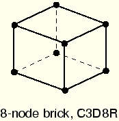
Displacements and rotations are calculated only at the nodes of the element. At any other point in the element, the displacements are obtained by interpolating from the nodal displacements. Elements that have nodes only at their corners, such as the 8-node brick shown in Figure 4–2, use linear interpolation in each direction and are often called linear elements or first-order elements. Elements with midside nodes are often called quadratic or second-order elements. In ABAQUS/Explicit all elements are first-order except for the quadratic triangle and tetrahedron, which use a modified second-order interpolation.
Typically, the number of nodes in an element is clearly identified in the element name. The 8-node brick element, as you have seen, is called C3D8R; and the 4-node general shell element is called S4R. The beam element family uses a different convention, wherein the order of interpolation is identified in the name. Thus, a first-order, three-dimensional beam element is called B31.
Formulation
An element's formulation refers to the mathematical theory used to define the element's behavior. In the absence of adaptive meshing all of the deformable elements in ABAQUS/Explicit are based on the Lagrangian or material description of behavior: the element deforms with the material. In the alternative Eulerian, or spatial, description elements are fixed in space as the material flows through them. Adaptive meshing in ABAQUS/Explicit combines the features of pure Lagrangian and Eulerian analyses and allows the motion of the element to be independent of the material; it is not discussed in this guide.
Integration
ABAQUS uses numerical techniques to integrate various quantities over the volume of each element. For most elements ABAQUS uses Gaussian quadrature to evaluate the material response at each integration point in each element.
ABAQUS uses the letter “R” at the end of the element name to indicate reduced-integration elements. For example, CAX4R is the 4-node, reduced-integration, first-order, axisymmetric solid element.
Between the different element families, continuum or solid elements can be used to model the widest variety of components. Conceptually, continuum elements simply model small blocks of material in a component. Since they can be connected to other elements on any of their faces, continuum elements, like bricks in a building or tiles in a mosaic, can be used to build models of nearly any shape, subjected to nearly any loading. ABAQUS/Explicit has both stress/displacement and coupled temperature-displacement continuum elements; we will only discuss stress/displacement elements in this guide.
Continuum elements in ABAQUS have names that begin with the letter “C.” The next two letters indicate the dimensionality and the active degrees of freedom in the element. The letters “3D” indicate a three-dimensional element; “AX,” an axisymmetric element; “PE,” a plane strain element; and “PS,” a plane stress element.
Two-dimensional continuum element library
ABAQUS has several classes of two-dimensional continuum elements that differ from each other in their out-of-plane behavior. Two-dimensional elements can be quadrilateral (CPE4R, CPS4R, and CAX4R) or triangular (CPE3, CPE6M, CPS3, CPS6M, CAX3, and CAX6M). Figure 4–3 shows the three classes that are used most commonly.
Plane strain elements assume that the out-of-plane strain, ![]() , is zero; they can be used to model thick structures.
, is zero; they can be used to model thick structures.
Plane stress elements assume that the out-of-plane stress, ![]() , is zero; they are suitable for modeling thin structures.
, is zero; they are suitable for modeling thin structures.
Axisymmetric elements, the “CAX” class of elements (CAX3, CAX4R, and CAX6M), model a 360° ring; they are suitable for analyzing structures with axisymmetric geometry subjected to axisymmetric loading.
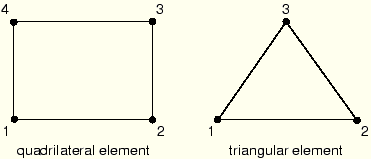
Two-dimensional solid elements must be defined in the 1–2 plane so that the node ordering is counterclockwise around the element perimeter, as shown in Figure 4–4.
When using a preprocessor to generate the mesh, ensure that the element normals all point in the same direction as the positive, global 3-axis. Failure to provide the correct element connectivity will cause ABAQUS to issue an error message stating that elements have negative volume.Three-dimensional continuum element library
Three-dimensional continuum elements can be hexahedra (C3D8R), wedges (C3D6), or tetrahedra (C3D4 and C3D10M).
Whenever possible hexahedral elements (C3D8R) or second-order tetrahedral elements (C3D10M) should be used. First-order tetrahedra (C3D4) have a simple, constant-strain formulation and very fine meshes are required for an accurate solution.
Degrees of freedom
All of the continuum elements have translational degrees of freedom at each node. Correspondingly, degrees of freedom 1, 2, and 3 are active in three-dimensional elements, while only degrees of freedom 1 and 2 are active in plane strain elements, plane stress elements, and axisymmetric elements.
Element properties
The *SOLID SECTION option defines the material and any additional geometric data associated with a set of continuum elements. For three-dimensional and axisymmetric elements no additional geometric information is required: the nodal coordinates completely define the element geometry. For plane stress and plane strain elements the thickness of the elements must be specified on the data line. For example, if the elements are 0.2 m thick, the element property definition would be the following:
*SOLID SECTION, ELSET=<element set name>, MATERIAL=<material name>
0.2,
Integration
Each first-order continuum element in ABAQUS/Explicit has a single integration point. For first-order triangular, tetrahedral, and wedge elements having one integration point is considered to be full integration, while for quadrilateral and hexahedral (brick) elements having one integration point is considered to be reduced integration. The second-order elements in ABAQUS/Explicit have either three or four integration points, depending on whether they are two- or three-dimensional; this is considered to be full integration.
Element output variables
By default, element output variables such as stress and strain reference the global Cartesian coordinate system. Thus, the ![]() component of stress at the integration point shown in Figure 4–5(a) acts in the global 1-direction. Even if the element rotates during a simulation, as shown in Figure 4–5(b), the default is still to use the global Cartesian system as the basis for defining the element variables.
component of stress at the integration point shown in Figure 4–5(a) acts in the global 1-direction. Even if the element rotates during a simulation, as shown in Figure 4–5(b), the default is still to use the global Cartesian system as the basis for defining the element variables.
Shell elements are used to model structures in which one dimension (the thickness) is significantly smaller than the other dimensions and the stresses in the thickness direction are negligible.
Shell element names in ABAQUS begin with the letter “S.” The axisymmetric shell begins with the letters “SAX.” The first number in a shell element name indicates the number of nodes in the element, except for the case of axisymmetric shells, for which the first number indicates the order of interpolation. All shell elements in ABAQUS/Explicit account for finite membrane strains and arbitrarily large rotations with the following exceptions: if the element name ends with the letter “S,” the element uses a small-strain formulation and does not consider warping. If the element name ends with the letters “SW,” the element uses a small-strain formulation but considers warping.
Conventional versus continuum shell elements
Two types of shell elements are available in ABAQUS: conventional shell elements and continuum shell elements. Conventional shell elements discretize a reference surface by defining the element's planar dimensions, its surface normal, and its initial curvature. The nodes of a conventional shell element, however, do not define the shell thickness; the thickness is defined through section properties. Continuum shell elements, on the other hand, resemble three-dimensional solid elements in that they discretize an entire three-dimensional body yet are formulated so that their kinematic and constitutive behavior is similar to conventional shell elements. Continuum shell elements are more accurate in contact modeling than conventional shell elements, since they employ two-sided contact taking into account changes in thickness. For thin shell applications, however, conventional shell elements provide superior performance.
In this manual only conventional shell elements are discussed. Henceforth, we will refer to them simply as “shell elements.” For more information on continuum shell elements, see “Shell elements: overview,” Section 15.6.1 of the ABAQUS Analysis User's Manual.
Shell element library
Triangular and quadrilateral elements are available with linear interpolation and your choice of large-strain and small-strain formulations. A linear axisymmetric shell element is available.
For most analyses the standard large-strain shell elements (S4R, S3R, and SAX1) are appropriate. If, however, the analysis involves small membrane strains and arbitrarily large rotations, the small-strain shell elements (S4RS, S3RS, and S4RSW) are more computationally efficient.
Degrees of freedom
The three-dimensional shell elements (S3R, S4R, S3RS, S4RS, and S4RSW) have six degrees of freedom at each node (three translations and three rotations).
The axisymmetric shell (SAX1) has three degrees of freedom at each node:
Element properties
Use either the *SHELL GENERAL SECTION or the *SHELL SECTION option to define the thickness and material properties for a set of shell elements. These two options have similar formats:
*SHELL SECTION, ELSET=<element set name>, MATERIAL=<material name>
<thickness>, <number of section points>
or
*SHELL GENERAL SECTION, ELSET=<element set name>,
MATERIAL=<material name>
<thickness>,
If you specify the *SHELL SECTION option, ABAQUS uses numerical integration to calculate the behavior at selected points (called section points) through the thickness of the shell, as shown in Figure 4–6. The MATERIAL parameter references a material property definition, which may be linear or nonlinear. You can specify any odd number of section points through the shell thickness.
The *SHELL GENERAL SECTION option allows you to define the cross-section behavior in a number of general ways to model linear or nonlinear behavior. Since ABAQUS models the shell's cross-section behavior directly in terms of section engineering quantities (area, moments of inertia, etc.) with this option, there is no need for ABAQUS to integrate any quantities over the element cross-section. Therefore, *SHELL GENERAL SECTION is less expensive computationally than *SHELL SECTION. The response is calculated in terms of force and moment resultants; the stresses and strains are calculated only when they are requested for output.
Reference surface offsets
The reference surface of the shell is defined by the shell element's nodes and normal definitions. When modeling with shell elements, the reference surface is typically coincident with the shell's midsurface. However, many situations arise in which it is more convenient to define the reference surface as offset from the shell's midsurface. For example, surfaces created in CAD packages usually represent either the top or bottom surface of the shell body. In this case it may be easier to define the reference surface to be coincident with the CAD surface and, therefore, offset from the shell's midsurface.
Shell offsets can also be used to define a more precise surface geometry for contact problems where shell thickness is important. By default, shell offset and thickness are accounted for in contact constraints in ABAQUS/Explicit. The effect of offset and thickness in contact can be suppressed, if required.
Shell offsets can also be useful when modeling a shell with continuously varying thickness. In this case defining the nodes at the shell midplane can be difficult. If one surface is smooth while the other is rough, as in some aircraft structures, it is easiest to use shell offsets to define the nodes at the smooth surface.
Offsets can be introduced by using the OFFSET parameter on the *SHELL SECTION and *SHELL GENERAL SECTION options. The offset value is defined as a fraction of the shell thickness measured from the shell's midsurface to the shell's reference surface.
The degrees of freedom for the shell are associated with the reference surface. All kinematic quantities, including the element's area, are calculated there. Large offset values for curved shells may lead to a surface integration error, affecting the stiffness, mass, and rotary inertia for the shell section. For stability purposes ABAQUS/Explicit also automatically augments the rotary inertia used for shell elements on the order of the offset squared, which may result in errors in the dynamics for large offsets. When large offsets from the shell's midsurface are necessary, use multi-point constraints or rigid body constraints instead.
Element output variables
The element output variables for shells are defined in terms of local material directions that lie on the surface of each shell element. These axes rotate with the element's deformation.
Beam elements are used to model components in which one dimension (the length) is significantly greater than the other two dimensions and only the stress in the direction along the length of the beam is significant.
Beam element names in ABAQUS begin with the letter “B.” The next character indicates the dimensionality of the element: “2” for two-dimensional beams and “3” for three-dimensional beams. The third character indicates the interpolation used: “1” for linear interpolation and “2” for quadratic interpolation. Linear beams (B21 and B31) and quadratic beams (B22 and B32) are available in two and three dimensions.
Degrees of freedom
Three-dimensional beams have six degrees of freedom at each node: three translational degrees of freedom (1–3) and three rotational degrees of freedom (4–6).
Two-dimensional beams have three degrees of freedom at each node: two translational degrees of freedom (1 and 2) and one rotational degree of freedom (6) about the normal to the plane of the model.
Element properties
Use the *BEAM SECTION option to define the geometry of the beam cross-section; the nodal coordinates define only the length. The beam cross-section is defined geometrically, and the MATERIAL parameter refers to a material property definition. ABAQUS calculates the cross-section behavior of the beam by numerical integration over the cross-section, allowing both linear and nonlinear material behavior.
Formulation and integration
The beams are shear deformable and account for finite axial strains; therefore, they are suitable for modeling both slender and non-slender beams.
Element output variables
The stress components in three-dimensional beam elements are the axial stress (![]() ) and the shear stress due to torsion (
) and the shear stress due to torsion (![]() ). The shear stress acts about the section wall in a thin-walled section. Corresponding strain measures are also available, as well as estimates of transverse shear forces on the section.
). The shear stress acts about the section wall in a thin-walled section. Corresponding strain measures are also available, as well as estimates of transverse shear forces on the section.
The two-dimensional beams use only axial stress and strain.
The axial force, bending moments, and curvatures about the local beam axes can also be requested for output. For details of what components are available with which elements, refer to the ABAQUS Analysis User's Manual
Truss elements are rods that can carry only tensile or compressive loads. They have no resistance to bending; therefore, they are useful for modeling pin-jointed frames. Moreover, truss elements can be used as an approximation for cables or strings (for example, in a tennis racket). Trusses are also sometimes used to represent reinforcement within other elements.
The truss element names begin with the letter “T.” The next two characters indicate the dimensionality of the element—“2D” for two-dimensional trusses and “3D” for three-dimensional trusses. The final character represents the number of nodes in the element. Linear truss elements (T2D2 and T3D2) are available in two and three dimensions.
Degrees of freedom
Truss elements have only translational degrees of freedom at each node. Three-dimensional truss elements have degrees of freedom 1, 2, and 3, while two-dimensional truss elements have degrees of freedom 1 and 2.
Element properties
The *SOLID SECTION option is used to specify the name of the material property definition associated with the given set of truss elements. The cross-sectional area is given on the data line:
*SOLID SECTION, ELSET=<element set>, MATERIAL=<material>
<cross-sectional area>
Element output variables
Axial stress and strain are available as output.
These elements (MASS and ROTARYI) define mass and rotary inertia at a discrete point.
Degrees of freedom
Mass elements have three translational degrees of freedom at each node. Rotary inertia elements have three rotational degrees of freedom at each node.
Element properties
Use the *MASS option to define the element property for a mass element:
*MASS, ELSET=<element set name>
<mass magnitude>,
Use the *ROTARY INERTIA option to define the element properties for a rotary inertia element:
*ROTARY INERTIA, ELSET=<element set name>
<I11>, <I22>, <I33>,<I12>, <I13>, <I23>
Element output variables
No output is available for these elements.
Spring and dashpot elements (SPRINGA and DASHPOTA) are used to model the effective stiffness or damping between two nodes without modeling the bodies in detail. The line of action remains between the two nodes throughout the deformation.
Degrees of freedom
Spring and dashpot elements have three translational degrees of freedom at each node.
Element properties
Use the *SPRING option to define the linear or nonlinear element properties for a spring element. To be consistent with SPRINGA and DASHPOTA elements in ABAQUS/Standard, the first data line following *SPRING and *DASHPOT is blank. If defining a linear spring, use the following:
*SPRING, ELSET=<element set name>

<spring stiffness>,
If defining a nonlinear spring, use the following, repeating the second data line as often as necessary:
*SPRING, ELSET=<element set name>, NONLINEAR

<force>, <relative displacement>
Use the *DASHPOT option to define the linear or nonlinear element properties for a dashpot element. If defining a linear dashpot, use the following:
*DASHPOT, ELSET=<element set name>

<dashpot coefficient>,
If defining a nonlinear dashpot, use the following, repeating the second data line as often as necessary:
*DASHPOT, ELSET=<element set name>, NONLINEAR

<force>, <relative velocity>
Element output variables
For spring elements S11 is the force in the spring, and E11 is the relative displacement across the spring. For dashpot elements S11 is the force in the dashpot, and E11 is the relative displacement across the dashpot.