Some element types fall outside the stability calculations performed by ABAQUS/Explicit. The following elements have the potential to destabilize an analysis:
Spring elements
Dashpot elements
Mass elements
Rotary inertia elements
Hydrostatic fluid elements
Elements that are part of a rigid body
We will use simple models to illustrate instabilities in ABAQUS/Explicit. While the program has been designed to provide efficient and stable solutions in almost all cases, there are some unusual situations involving springs and dashpots in which a solution may become unstable. It is useful to be able to recognize such instabilities when they occur.
The following example uses very simple models to illustrate stability problems that could also occur in larger, more complex models. Once you understand how to determine whether these simple analyses have become unstable, you can then use the same methods to determine whether your own engineering analyses have become unstable. With larger models it is necessarily more difficult to determine ahead of time whether or not the analysis will become unstable because the locations and loadings on the springs and dashpots become a factor. For example, an analysis that might have otherwise become unstable could be subjected to a contact constraint that keeps the instability from occurring.
Springs, as well as elements such as continuum elements, impose certain stability requirements on an analysis. Each element has its own maximum stable time increment based on the stiffness and mass associated with the element. Since a spring element has stiffness but no mass of its own, mass is associated with a spring element through its connection to other elements containing mass. If a spring element is connected to continuum elements, for example, it generally is not possible to determine what mass is associated with the spring element. Therefore, it is not possible for ABAQUS/Explicit to calculate the stable time increment for a spring element. If the stable time increment required by the spring is smaller than the smallest stable time increment of the rest of the model, the spring defines the controlling stable time increment for the model, and the analysis may become unstable.
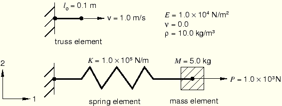
The model shown in Figure 3–17 is made up of two separate, simple bodies: a single truss element and a spring element with a mass element at the free end. The left-hand side of both bodies is fixed, while the right-hand side is loaded. Since the truss element has both stiffness and mass, ABAQUS/Explicit determines a stable time increment for the truss element. Since the spring element has stiffness but no mass, ABAQUS/Explicit does not calculate a stable time increment for the spring element. Likewise, ABAQUS/Explicit does not calculate a stable time increment for the mass element, which has mass but no stiffness. The details of the input file corresponding to this model are not discussed here; the input file itself can be found in “Potential instabilities with springs and dashpots,” Section A.3.
In this simple example, however, we can calculate the stability requirements of the spring-mass system analytically because the mass associated with the spring is simply the mass of the mass element. Since the spring stiffness and associated mass are constant throughout the analysis, the maximum stable time increment for the spring-mass system is also constant. The stable time increment for the truss, however, changes throughout the analysis, as the length and, thus, the stiffness of the truss changes. At the start of the analysis the stable time increment for the truss is smaller than that required for the spring-mass system. As the truss stretches, its stable time increment increases, and eventually the stable time increment for the spring-mass system becomes the controlling factor in the analysis. When the stable time increment for the analysis as determined by the truss becomes greater than that required by the spring-mass system, the analysis becomes unstable. The stable time increment versus time is illustrated in Figure 3–18.
The spring-mass system is loaded dynamically with a constant force of 1000 N, causing the mass to accelerate and the spring to stretch. Since the force is applied as a step function, the spring will oscillate according to the applied force and the mass, and the stiffness of the spring. With a spring stiffness of 1 × 10⁵ N/m and a force of 1 × 10³ N, the average displacement of the spring is 0.01 m, and the maximum displacement is 0.02 m. We can calculate the stable time increment for the spring-mass system just as we would for any other element. Recall that the stable time increment of an element is related to its frequency, according to the following relation:
![]()
![]()
![]()
![]()
![]()
![]()
The truss stretches with a constant velocity of 1.0 m/s; thus, the length of the truss element at any given time is
![]()
![]()
Fetch the input file stability.inp, and run the analysis. Examine the contents of the status (.sta) file, and plot the displacement history of the spring's free end and the energy history of the model to determine the source of the instability.
Status file
The output from the analysis provides us with several indications that the analysis has become unstable. The status file is particularly useful and would contain information similar to the following:
.
.
.
 -------------------------------------------------------------------------------
  STABLE TIME INCREMENT INFORMATION
 -------------------------------------------------------------------------------


   The stable time increment estimate for each element is based on
   linearization about the initial state.


    Initial time increment = 3.13066E-03

    Statistics for all elements:
       Mean = 3.13066E-03
       Standard deviation = 0.0000

    Most critical elements :
     Element number   Rank    Time increment   Increment ratio
    ----------------------------------------------------------
            3          1       3.130655E-03      1.000000E+00


 The single precision ABAQUS/Explicit executable will be used in this analysis.


 -------------------------------------------------------------------------------
  SOLUTION PROGRESS
 -------------------------------------------------------------------------------

  STEP 1  ORIGIN 0.0000

   Total memory used for step 1 is approximately 41.8 kilowords
   Global time estimation algorithm will be used.
   Scaling factor :  1.0000
   Percentage change in total mass at the start of step:  0.0000

             STEP      TOTAL       CPU     STABLE      CRITICAL  KINETIC
  INCREMENT  TIME      TIME        TIME   INCREMENT    ELEMENT   ENERGY    MONITOR
         0  0.000E+00 0.000E+00   00:00:00 3.131E-03       3   2.500E-01 0.000E+00
 Results number  0 at increment zero.
 ODB Field Frame Number    0 of    1 requested intervals at increment zero.
        20  1.005E-01 1.005E-01   00:00:00 9.438E-03       3   6.271E+00 1.561E-02
        28  2.052E-01 2.052E-01   00:00:00 1.645E-02       3   1.563E+02 9.990E-02

 ***WARNING: Large rotation detected for SPRINGA element 1. The analysis may go
             unstable. This message is printed during the first applicable
             increment, but will not be printed during subsequent increments
             for the remainder of the step.


 ***WARNING: Large rotation is detected in 1 1D element (truss, spring, or
             dashpot). The analysis may go unstable.

        34  3.106E-01 3.106E-01   00:00:00 1.913E-02       3   6.906E+06-2.566E+01
        39  4.107E-01 4.107E-01   00:00:00 2.136E-02       3   1.393E+14 1.352E+05
 Results Number  1 at 0.41073
        44  5.220E-01 5.220E-01   00:00:00 2.360E-02       3   7.129E+22-3.497E+09

.
.
.
For this analysis we suspected in advance that the spring-mass system would become unstable; therefore, we selected the right-hand node of the spring as the monitor node. The data in the monitor column are, therefore, the displacement of the mass element. The first few increments show that the mass has a displacement, as expected, between 0 m and 0.02 m. However, in increment 28 at a time of 0.2052 s the displacement of node 2 has become 0.099 m, well outside the correct range. We anticipated that the spring-mass system would become unstable once the time exceeded 0.169 s, and increment 28 is the first increment in the status file beyond a time of 0.169 s. Between increments 28 and 34 the displacement of the mass remains negative and the first warning messages regarding analysis stability appear. In this case the warning indicates that the SPRINGA element has undergone a large rotation. This rotation does not refer to a rotational degree of freedom (which spring elements do not possess) but rather a rigid rotation of the spring that has occured because the mass is displaced in the negative direction (the spring has effectively turned inside out). Beyond increment 34 the displacement of the mass increases rapidly to a value of –3.497 × 10⁹ m in increment 44.
Displacement history
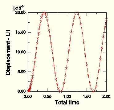
The displacement history of the spring's free end is shown graphically in Figure 3–19. Notice that the distance increases between subsequent symbols on the displacement history plot, indicating that the time increment used by ABAQUS/Explicit increases throughout the analysis. It is clear from the unrealistic displacements that the spring-mass system has become unstable.
Using energy to determine instability
In a more complicated analysis you may not know ahead of time which parts of the model are likely to become unstable. You must then have other means of determining whether or not the solution has become unstable besides monitoring the displacements at a single node. The kinetic energy shown for each increment in the status file provides another simple indication of stability. The advantage of checking the kinetic energy over monitoring a particular degree of freedom is that the kinetic energy shown in the status file is the summation of the kinetic energy over the entire model. An unrealistic growth in the kinetic energy may indicate that the analysis has become unstable but does not indicate the problem area. In this example the kinetic energy starts to grow unrealistically at the same time that the stretch in the spring becomes unrealistic, indicating that the two effects have the same cause.
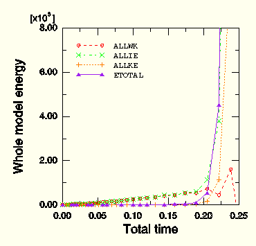
The energies are useful indications of the solution stability, and the most general way to view the energies is to create history plots in ABAQUS/Viewer. Figure 3–20 shows the history of the energy balance (ETOTAL), the kinetic and internal energies (ALLKE, ALLIE), as well as the external work (ALLWK).
Up to approximately 0.16 s the energy balance remains nearly constant at zero. A constant energy balance is an indication that the solution is stable; conversely, a grossly nonconstant energy balance strongly suggests that the solution is unstable. The energy plots show that when the time reaches 0.16 s, the energy balance increases dramatically, as do the other energies.
Three methods of removing the instability are discussed in the following sections.
Adding mass
The preferred method of removing an instability caused by springs is to increase the mass associated with the springs. Usually, springs are used to model stiffness without modeling the more complex response of the associated continuum. Springs can model the stiffness accurately, but they do not account for the mass. The natural frequency of the spring-mass system decreases as the mass associated with the spring increases; correspondingly, the stable time increment of the spring-mass system increases. If enough mass is added to the nodes associated with the spring, the stable time increment of the spring-mass system can be increased such that it will always be greater than the stable time increment of the rest of the model. At that level the spring will have the desired effect on the behavior of the structure without controlling the stability of the analysis.
We can calculate the mass necessary to add to the right-hand node of the spring element so that the spring-mass system remains stable throughout the analysis, which lasts 2 seconds. As shown previously, by the end of the step the stable time increment for the truss has increased to
![]()
![]()
![]()
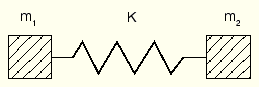
In a real analysis springs can be used not only to connect a structure to ground (a fixed boundary condition), as shown previously, but also to connect one part of a structure to another part. In such a model both ends of the spring are free to move, as shown in Figure 3–22.
Both ends may require additional mass for numerical stability. The natural frequency for this case is
![]()
![]()
![]()
![]()
![]()
The effect of damping
Dashpot elements are often used in conjunction with spring elements to provide damping at discrete points within a model. Using dashpots requires some caution and understanding of the effects of damping on stability. As with springs, dashpots affect the stable time increment of the analysis, yet ABAQUS/Explicit does not consider dashpots when calculating the stable time increment. In fact, a dashpot in parallel with a spring always lowers the actual stable time increment of the spring. On the other hand, ABAQUS/Explicit does consider the effects of material damping on the stable time increment.
With no material damping
![]()
![]()
The stable time increment for case ![]() is always less than it is for case
is always less than it is for case ![]() . Generally, it is not possible to calculate
. Generally, it is not possible to calculate ![]() because you do not know the value for critical damping. Therefore, it is difficult to determine ahead of time at what value of
because you do not know the value for critical damping. Therefore, it is difficult to determine ahead of time at what value of ![]() an analysis will become unstable.
an analysis will become unstable.
Table 3–4 summarizes the mass that should be added to spring and spring-dashpot systems to ensure stability up to the desired time increment. For simplicity, the spring-dashpot systems are solved for ![]() instead of
instead of ![]() .
.
Controlling the time incrementation
If adding mass to the spring nodes is not physically appropriate, you can retain stability by controlling the time incrementation. The *DYNAMIC, EXPLICIT option offers several useful parameters. The FIXED TIME INCREMENTATION parameter causes ABAQUS/Explicit to persist with the stable time increment that was calculated at the start of the analysis. In this example using the FIXED TIME INCREMENTATION parameter eliminates the instability from the solution because the stable time increment is not permitted to increase beyond the initial, stable level. To include an additional factor of safety, you can set the SCALE FACTOR parameter to the desired value.