The starting point for each general step is the deformed state at the end of the last general step. Therefore, the state of the model evolves in a sequence of general steps as it responds to the loads defined in each step. The initial conditions specified using the *INITIAL CONDITIONS option define the starting point for the first general step in the simulation.
All general analysis procedures share the same concepts for applying loads and defining “time.”
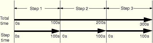
ABAQUS has two measures of time in a simulation. The total time increases throughout all general steps and is the accumulation of the total step time from each general step. Each step also has its own time scale (known as the step time), which begins at zero for each step. Time varying loads and boundary conditions can be specified in terms of either time scale. The time scales for an analysis whose history is divided into three steps, each 100 seconds long, are shown in Figure 10–1.
In general steps the loads must be specified as total values, not incremental values. For example, if a concentrated load has a value of 1000 N in the first step and it is increased to 3000 N in the second general step, the magnitude given on the *CLOAD option in the two steps should be 1000 N and 3000 N, not 1000 N and 2000 N.
Modifying loads from step to step
Applying a load in ABAQUS requires more than just providing its magnitude and direction. You must also specify how these new loads interact with the existing loads and boundary conditions of the same type that were defined in previous general steps. All the loading and boundary condition options—such as *BOUNDARY, *CLOAD, and *DLOAD—use the OP parameter to indicate how the loads they define interact with the existing loads of that type. The parameter can be set to OP=MOD or OP=NEW. ABAQUS assumes OP=MOD if no value is provided for the OP parameter.
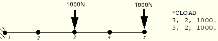
Using OP=MOD causes the loads defined in the current general step to modify the same types of loads already applied to the model in previous general steps. Any load that is not specifically modified in the current step continues to follow its associated amplitude definition, provided the amplitude curve is defined in terms of total time; otherwise, the load is maintained at the magnitude it had at the end of the last general step. For example, consider a cantilever beam modeled with two B22 elements (see Figure 10–2) with concentrated loads of 1000 N applied to nodes 3 and 5 in the first general step.
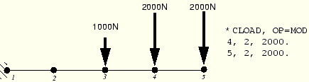
In the next general step (Step 2) loads of 2000 N are specified on nodes 4 and 5 using the OP=MOD parameter. Thus, these loads modify those applied in Step 1. The loading applied to the model at the end of Step 2 is shown in Figure 10–3.
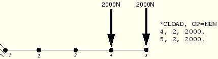
Using OP=NEW causes ABAQUS to remove all existing loads of that type and only apply the loads specified in this current step to the model. If OP=NEW is specified on the *CLOAD option in Step 2, the loading on our example beam is shown in Figure 10–4.
Be very careful when you use the OP=NEW parameter on the *BOUNDARY option to remove a boundary constraint from your model. All boundary constraints are removed from the model, not just the one you want removed; therefore, you must respecify all the boundary conditions that should remain active in the model. Remember that the boundary conditions that you specify must provide enough constraints to prevent rigid body motions in all components of your model. Failure to do so will cause ABAQUS to issue numerical singularity warnings and leads to excessive displacements.