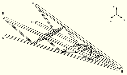
A light-service, cargo crane is shown in Figure 6–11. You have been asked to determine the deflections of the crane when it carries a load of 10 kN. You should also identify the critical members and joints in the structure: i.e., those with the highest stresses and loads.
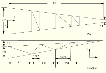
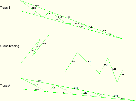
The crane consists of two truss structures joined together by cross bracing. The two main members in each truss structure are steel box beams (box cross-sections). Each truss structure is stiffened by internal bracing, which is welded to the main members. The cross bracing connecting the two truss structures is bolted to the truss structures. These connections can transmit little, if any, moment and, therefore, are treated as pinned joints. Both the internal bracing and cross bracing use steel box beams with smaller cross-sections than the main members of the truss structures. The two truss structures are connected at their ends (at point E) in such a way that allows independent movement in the 3-direction and all of the rotations, while constraining the displacements in the 1- and 2-directions to be the same. The crane is welded firmly to a massive structure at points A, B, C, and D. The dimensions of the crane are shown in Figure 6–12. In the following figures, truss A is the structure consisting of members AE, BE, and their internal bracing; and truss B consists of members CE, DE, and their internal bracing.
The ratio of the typical cross-section dimension to global axial length in the main members of the crane is much less than 1/15. The ratio is approximately 1/15 in the shortest member used for internal bracing. Therefore, it is valid to use beam elements to model the crane.
You should use the default global rectangular Cartesian coordinate system shown in Figure 6–11 and Figure 6–12. Locate the origin of the coordinate system midway between points A and D. If you build your model with a different origin or orientation of the coordinate system, ensure that the input data in your model reflect your coordinate system and not the one shown here.
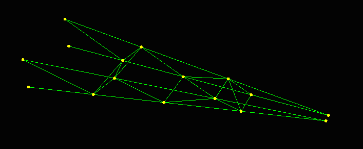
The cargo crane will be modeled with three-dimensional, slender, cubic beam elements (B33). The cubic interpolation in these elements allows us to use a single element for each member and still obtain accurate results under the applied bending load. The mesh that you should use in the simulation is shown in Figure 6–13.
The welded joints in the crane provide complete continuity of the translations and rotations from one element to the next. You, therefore, need only a single node at each welded joint in the model. The bolted joints, which connect the cross bracing to the truss structures, and the connection at the tip of the truss structures are different. Since these joints do not provide complete continuity for all nodal degrees of freedom, separate nodes are needed for each element at the connection. Appropriate constraints between these separate nodes must then be given by using the *MPC, *BOUNDARY, or *EQUATION options. The *MPC and *EQUATION options are discussed in more detail later.
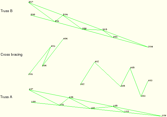
The node numbers for the various members of the cargo crane model are shown in Figure 6–14.
These are the node numbers from the input file given in “Cargo crane,” Section A.4. Separate nodes have been defined on the cross-bracing elements and the truss structures that they connect. Separate nodes are also needed at the end of each truss structure, point E in Figure 6–11. The node numbers in your model may be different from those shown here.The element numbers for the various members of the cargo crane model are shown in Figure 6–15.
These are the element numbers from the input file given in “Cargo crane,” Section A.4. The element numbers in your model may be different from those shown here.While you can generate the mesh for this simulation using a preprocessor, you may find it easier to build this model with an editor. The ABAQUS input options used to create the nodes and elements shown on the preceding pages can be found in “Cargo crane,” Section A.4. If you do use a preprocessor, most likely you will have to modify the input data to ensure correct modeling of the joints between members and correct orientation of the beam element cross-sections. If you wish to create the entire model using ABAQUS/CAE, refer to “Example: cargo crane,” Section 6.4 of Getting Started with ABAQUS.
At this point we assume that you have created the basic mesh either by using a preprocessor or with an editor. In this section you will review and make corrections to your input file, as well as include additional information, such as beam section properties and orientations.
Heading
Use a suitable, descriptive heading in your input file, such as the following:
*HEADING
3-D model of light-service cargo crane
S.I. Units (m, kg, N, sec)
Nodal coordinates and element connectivity
Define the nodal coordinates in a *NODE option block. If you decide to do this with an editor, you may want to use the mesh generation commands found in “Cargo crane,” Section A.4. Create a node set called ATTACH containing the nodes at points A, B, C, and D, the points at which the crane is attached to the parent structure.
*NSET, NSET=ATTACH
100,107,200,207
Create elements in your model that correspond to the elements shown in Figure 6–15, but remember that your numbering may be different. (Having the same numbering will make defining some modeling features easier, however.) There are several element sets that you will need in this simulation. As you define the elements, group them into the following element sets:
OUTA	    100, 101, 102, 103, 104, 105, 106
BRACEA	  110, 111, 112, 113, 114
OUTB	    200, 201, 202, 203, 204, 205, 206
BRACEB	  210, 211, 212, 213, 214
CROSSEL	 300, 301, 302, 303, 304, 305, 306, 307
where these element numbers refer to those elements shown in Figure 6–15. The element sets OUTA and OUTB contain the main outer members for the two truss structures. Element sets BRACEA and BRACEB contain the elements modeling the internal bracing within each truss structure. Element set CROSSEL contains the cross bracing that connects the two truss structures.
Beam element properties
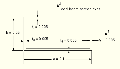
Since the material behavior in this simulation is assumed to be linear elastic, use the *BEAM GENERAL SECTION option to define the section properties. All of the beams in this structure have a box-shaped cross-section.
A box-section is specified using the parameter SECTION=BOX. The first data line contains the section dimensions, which are the dimensions ![]() ,
, ![]() ,
, ![]() ,
, ![]() ,
, ![]() , and
, and ![]() shown in Figure 6–16 for a box section. The dimensions shown in Figure 6–16 are for the main members of the two trusses in the crane.
shown in Figure 6–16 for a box section. The dimensions shown in Figure 6–16 are for the main members of the two trusses in the crane.
The beam section axes for the main members should be oriented such that the beam 1-axis is orthogonal to the plane of the truss structures shown in the elevation view (Figure 6–12) and the beam 2-axis is orthogonal to the elements in that plane. Specify this orientation by giving the approximate direction of the beam 1-axis (the ![]() -vector) on the second data line of the *BEAM GENERAL SECTION option. To get the correct normal,
-vector) on the second data line of the *BEAM GENERAL SECTION option. To get the correct normal, ![]() , in this case, you need to provide a very accurate
, in this case, you need to provide a very accurate ![]() . It is somewhat easier to provide an approximate direction, which would be the negative 3-direction. However, given the logic that ABAQUS uses to determine
. It is somewhat easier to provide an approximate direction, which would be the negative 3-direction. However, given the logic that ABAQUS uses to determine ![]() given
given ![]() and
and ![]() , the normal
, the normal ![]() is rotated slightly from its proper orientation if we use this approximate
is rotated slightly from its proper orientation if we use this approximate ![]() . You can specify the same
. You can specify the same ![]() -direction for all elements in each of the two truss structures. The third data line contains the elastic and shear moduli, assuming a mild strength steel with
-direction for all elements in each of the two truss structures. The third data line contains the elastic and shear moduli, assuming a mild strength steel with ![]() = 200.0 GPa,
= 200.0 GPa, ![]() = 0.25, and
= 0.25, and ![]() = 80.0 GPa. Add the following option blocks to your input file:
= 80.0 GPa. Add the following option blocks to your input file:
*BEAM GENERAL SECTION, SECTION=BOX, ELSET=OUTA
0.10,0.05,0.005,0.005,0.005,0.005
-0.1118, 0.0, -0.9936
200.E9,80.E9
*BEAM GENERAL SECTION, SECTION=BOX, ELSET=OUTB
0.10,0.05,0.005,0.005,0.005,0.005
-0.1118, 0.0, 0.9936
200.E9,80.E9
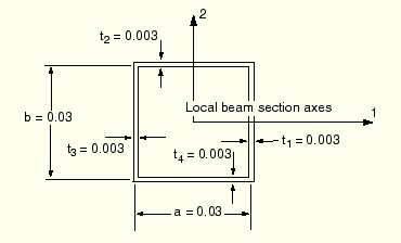
The dimensions of the beam sections for the bracing members are shown in Figure 6–17. Both the cross bracing and the bracing within each truss structure have the same beam section geometry, but they do not share the same orientation of the beam section axes. Therefore, separate *BEAM GENERAL SECTION options must be used. The bracing is made from the same steel as the main members.
The approximate ![]() -vector for the internal truss bracing is the same as for the main members of the respective truss structures. Use the following input to define the element properties of this bracing:
-vector for the internal truss bracing is the same as for the main members of the respective truss structures. Use the following input to define the element properties of this bracing:
*BEAM GENERAL SECTION, SECTION=BOX, ELSET=BRACEA
0.03,0.03,0.003,0.003,0.003,0.003
-0.1118, 0.0, -0.9936
200.E9,80.E9
*BEAM GENERAL SECTION, SECTION=BOX, ELSET=BRACEB
0.03,0.03,0.003,0.003,0.003,0.003
-0.1118, 0.0, 0.9936
200.E9,80.E9
We make some assumptions so that the orientation of the cross bracing is somewhat easier to specify. All of the beam normals (![]() -vectors) should lie approximately in the plane of the plan view of the cargo crane (see Figure 6–17). This plane is skewed slightly from the global 1–3 plane. Again, a simple method for defining such an orientation is to provide an approximate
-vectors) should lie approximately in the plane of the plan view of the cargo crane (see Figure 6–17). This plane is skewed slightly from the global 1–3 plane. Again, a simple method for defining such an orientation is to provide an approximate ![]() -vector that is orthogonal to this plane on the element property options. The vector should be nearly parallel to the global 2-direction. Since the angle between the normals from one element to the next is always greater than 20°, the normals are not averaged at the nodes.
-vector that is orthogonal to this plane on the element property options. The vector should be nearly parallel to the global 2-direction. Since the angle between the normals from one element to the next is always greater than 20°, the normals are not averaged at the nodes.
Depending on the exact orientation of the members in the cross bracing, it is possible that we would have to define the normals individually for each of the cross-bracing elements. Such an exercise would be very similar to what you have already done by defining the normals for the two truss structures. Since the square cross-bracing members are subjected to primarily axial loading, their deformation is not sensitive to cross-section orientation. Therefore, we accept the default normals that ABAQUS calculates to be correct. The approximate ![]() -vector for the cross bracing is aligned with the y-axis. Add the following option block to your model:
-vector for the cross bracing is aligned with the y-axis. Add the following option block to your model:
*BEAM GENERAL SECTION, SECTION=BOX, ELSET=CROSSEL
0.03,0.03,0.003,0.003,0.003,0.003
0.0,1.0,0.0
200.E9,80.E9
Beam section orientation
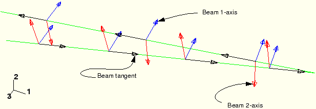
In this model you will have a modeling error if you provide data that only define the orientation of the approximate ![]() -vector. The averaging of beam normals at the nodes (see “Beam element curvature,” Section 6.1.3) causes ABAQUS to use incorrect geometry for the cargo crane model. To see this, you can use ABAQUS/Viewer to display the beam section axes and beam tangent vectors (see “Postprocessing,” Section 6.4.7). However, the normals in the crane model appear to be correct in ABAQUS/Viewer; yet, they are, in fact, slightly incorrect. You can also find such modeling mistakes by examining the averaged nodal normals that are printed in the data (.dat) file. Some of the normals in the incorrect model of the cargo crane are shown in the following output:
-vector. The averaging of beam normals at the nodes (see “Beam element curvature,” Section 6.1.3) causes ABAQUS to use incorrect geometry for the cargo crane model. To see this, you can use ABAQUS/Viewer to display the beam section axes and beam tangent vectors (see “Postprocessing,” Section 6.4.7). However, the normals in the crane model appear to be correct in ABAQUS/Viewer; yet, they are, in fact, slightly incorrect. You can also find such modeling mistakes by examining the averaged nodal normals that are printed in the data (.dat) file. Some of the normals in the incorrect model of the cargo crane are shown in the following output:
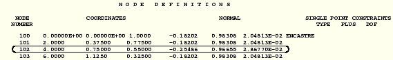
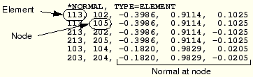
The problem is the normal vector for node 102, which does not match those at the other nodes defining the lower, main member in truss A (see Figure 6–14). Four elements (101, 102, 112, and 113) contain node 102. When the averaging of beam normals at nodes produces multiple independent normals, the additional normals at the node are also printed in the data file (see “Beam element curvature,” Section 6.1.3, for details). The correct geometry for the crane model requires three independent beam normals at node 102: one each for the bracing elements 112 and 113 and a single normal for elements 101 and 102. The normal shown above for node 102 is not the normal needed for elements 101 and 102. If it were, it would match the normals shown for nodes 100, 101, or 103. Nor is it the correct normal for either of the other two elements, whose normals are printed in the data file, as shown below.
                           N O R M A L   D E F I N I T I O N S

ELEMENT NODE           NORMAL             ELEMENT  NODE           NORMAL

 110    101  -0.2947  -0.9550  3.3161E-02   110    107  -0.2947  -0.9550   3.3161E-02
 111    101  -0.7581   0.6465  8.5304E-02   111    106  -0.7581   0.6465   8.5304E-02
 112    102  -0.2947  -0.9550  3.3161E-02   112    106  -0.2947  -0.9550   3.3161E-02
 114    103  -0.2947  -0.9550  3.3161E-02   114    105  -0.2947  -0.9550   3.3161E-02
In this table element 113 shows no normal for either of its nodes, node 102 and node 105. Thus, the normal shown for node 102 above in the NODE DEFINITIONS table was the average of the normals from elements 101, 102, and 113. Using the ABAQUS logic for averaging normals, we could have predicted that the normals at the nodes of element 113 would be averaged with the normals for the adjacent elements. For this problem the important part of the averaging logic is that normals that subtend an angle less than 20° with the reference normal are averaged with the reference normal to define a new reference normal. In the case of the normals at node 102, the original reference normal is the normal for elements 101 and 102. Since the normal for element 113 at node 102 subtends an angle less than 20° with the original reference normal, it is averaged with the normals for elements 101 and 102 at node 102 to define the new reference normal at that node. On the other hand, since the normal for element 112 subtends an angle of approximately 30° with the original reference normal, it has an independent normal at node 102, as shown in the data file.
This incorrect average normal means that elements 101, 102, and 113 have a section geometry that twists about the beam axis from one end of the element to the other, which is not the intended geometry. You must use the *NORMAL option to define the normals at node 102 for element 113 explicitly. Explicitly specifying the normal directions prevents ABAQUS from applying its averaging algorithm. You must also use *NORMAL for the corresponding elements on the opposite side of the crane: element 213, node 202 of truss B.
There is also a problem with the normals at nodes 104 and 204 at the tip of each truss structure, again because the angle between elements 103 and 104 is less than 20°. Since we are modeling straight beam elements, the normals are constant at both nodes in each element. Thus, the *NORMAL option block that you should put in your input file has six data lines. If you used the numbering scheme shown in Figure 6–14 and Figure 6–15, the following option block should be added to your input file:
Multi-point constraints
The cross bracing, unlike the internal truss bracing, is bolted to the truss members. You can assume that these bolted connections are unable to transmit rotations or torsion. The duplicate nodes that were defined at these locations are needed to define this constraint. In ABAQUS such constraints between nodes can be defined using multi-point constraints (MPCs) or constraint equations.
Multi-point constraints allow constraints to be imposed between different degrees of freedom of the model. A large library of MPCs is available in ABAQUS. (See “Linear constraint equations,” Section 20.2.1 of the ABAQUS Analysis User's Manual, for a complete list and a description of each one.) The format of the *MPC option is
*MPC
<type of MPC>,<node 1 or node set 1>,<node 2 or node set 2>, ......
You can define multiple constraints of the same type with just a single data line by using node sets. The MPC type needed to model the bolted connection is PIN. The pinned joint created by this MPC constrains the displacements at two nodes to be equal, but the rotations, if they exist at the nodes, remain independent.
There are many bolted joints in the crane model. The following is the complete *MPC option block for the model from “Cargo crane,” Section A.4:
*MPC
PIN,101,301
PIN,102,302
PIN,103,303
PIN,105,305
PIN,106,306
PIN,201,401
PIN,202,402
PIN,203,403
PIN,205,405
PIN,206,406
Add a similar option block to your model, changing the node numbers to correspond to those in your model. If all of the nodes on the two truss structures had been grouped into a node set called TRUSNODE and all of the nodes on the cross bracing had been grouped into a node set called CROSNODE, the option block could have been shortened to the following:
*NSET, NSET=TRUSNODE, UNSORTED
101,102,103,105,106,201,202,203,205,206
*NSET, NSET=CROSNODE, UNSORTED
301,302,303,305,306,401,402,403,405,406
*MPC
PIN, TRUSNODE, CROSNODE
If a node set is provided as the first item after the MPC type, the second item can be either another node set or a single node. When the data line of an *MPC option contains a node set and then a single node, as shown below, ABAQUS creates an MPC constraint between each node in the set and the individual node specified. For example, the following option block would create a pinned joint between node 301 and each node in node set TRUSNODE.
*MPC
PIN, TRUSNODE, 301
Constraint equations
Constraints between nodal degrees of freedom can also be specified with linear equations by using the *EQUATION option. The form of each equation is,
![]()
<Exactly four terms must be given on each data line except the final one, which can have fewer terms.>,<
>,<
>,<
>,<
>,<
>,
,<
>,<
>,<
>
In the crane model the tips of the two trusses are connected together such that degrees of freedom 1 and 2 (the translations in the 1- and 2-directions) are equal, while the other degrees of freedom (3–6) at the nodes are independent. We need two linear constraints, one equating degree of freedom 1 at node 104 to degree of freedom 1 at node 204:
![]()
![]()
Remember to change the node numbers if necessary for your model. The following option block defines the appropriate constraints at point E in the crane model (see Figure 6–11):
*EQUATION
2
104,1,1.0, 204,1,-1.0
2
104,2,1.0, 204,2,-1.0
The degrees of freedom at the first node defined in an *MPC or *EQUATION are eliminated from the stiffness matrix. Therefore, these nodes should not appear in other MPCs or constraint equations. Nor should boundary conditions be applied to the eliminated degrees of freedom.
Specify a static, linear perturbation simulation using the following options:
*STEP, PERTURBATION
Static tip load on crane
*STATIC
Boundary conditions
The crane is attached firmly to the parent structure. Use the following *BOUNDARY option block to constrain all of the nodes at the attachment points, which should have been grouped into node set ATTACH:
*BOUNDARY
ATTACH, ENCASTRE
Loading
A concentrated load of 10 kN is applied in the negative y-direction to node 104. Since there is a constraint equation connecting the y-displacement of nodes 104 and 204, the load is carried equally by both nodes. The *CLOAD option block that you should use is:
*CLOAD
104,2,-1.0E4
Output requests
Write the displacements (U) and reaction forces (RF) at the nodes, and the section forces (SF) in the elements to the output database for postprocessing with ABAQUS/Viewer. Also, print U, RF, and SF to the data file. Add the following option blocks to your input file:
*OUTPUT, FIELD
*NODE OUTPUT
U, RF
*ELEMENT OUTPUT
SF,
*NODE PRINT
U,
RF,
*EL PRINT
SF,
*END STEP
Store the input in a file called crane.inp. Run the analysis using the command
abaqus job=crane
Start ABAQUS/Viewer by typing
abaqus viewer odb=craneat the operating system prompt.
ABAQUS/Viewer displays a fast plot of the crane model.
Plotting the deformed model shape
To begin this exercise, plot the deformed shape.
To plot the deformed model shape:
From the main menu bar, select Plot![]() Deformed Shape; or use the
Deformed Shape; or use the ![]() tool in the toolbox to display the deformed model shape at the end of the analysis.
tool in the toolbox to display the deformed model shape at the end of the analysis.
From the main menu bar, select Options![]() Deformed Shape.
Deformed Shape.
The Deformed Shape Plot Options dialog box appears; by default, the Basic tab is selected.
Toggle on Superimpose undeformed plot.
Click OK.
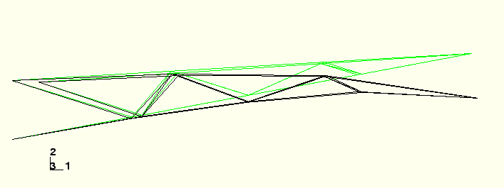
ABAQUS/Viewer displays an image of the deformed crane superimposed upon the undeformed crane.
Changing the view
The default view is isometric. You can change the view using the options in the View menu or the view tools on the toolbar.
To specify the view:
From the main menu bar, select View![]() Specify.
Specify.
The Specify View dialog box appears.
From the list of available methods, select Viewpoint.
Enter the X-, Y-, and Z-coordinates of the viewpoint vector as 0, 0, 1 and the coordinates of the up vector as 0, 1, 0.
Click OK.
ABAQUS/Viewer displays your model in the specified view.
Plotting individual element and node sets
You can use display groups in ABAQUS/Viewer to plot existing node and element sets. You will display only the elements in element set OUTA, the main members in truss structure A.
To display the elements in the element set OUTA:
From the main menu bar, select Tools![]() Display Group
Display Group![]() Create; or use the
Create; or use the ![]() tool in the toolbox.
tool in the toolbox.
The Create Display Group dialog box appears.
From the Item list in the top-left portion of this dialog box, select Elements.
From the Method list, select Element sets. A list of the available element sets appears in the right hand side of the dialog box. Select the element set PART-1-1.OUTA.
From the icons in the bottom portion of the dialog box, click ![]() to activate the Boolean Replace operation.
to activate the Boolean Replace operation.
Click Dismiss to close the dialog box.
ABAQUS/Viewer now displays only the elements in element set PART-1-1.OUTA.
Beam cross-section orientation
You can plot the section axes and beam tangents on the undeformed model shape.
To plot the beam section axes:
From the main menu bar, select Plot![]() Undeformed Shape; or use the
Undeformed Shape; or use the ![]() tool in the toolbox to display the undeformed model shape.
tool in the toolbox to display the undeformed model shape.
From the toolbar, click ![]() and select the isometric view from the Views dialog box that appears.
and select the isometric view from the Views dialog box that appears.
From the main menu bar, select Options![]() Undeformed Shape; then, click the Normals tab in the dialog box that appears.
Undeformed Shape; then, click the Normals tab in the dialog box that appears.
Toggle on Show normals, and accept the default setting of On elements.
In the Style area at the bottom of the Normals page, specify the Length to be Long.
Click OK.
The section axes and beam tangents are displayed on the undeformed shape.
Creating a hard copy
You can save the image of the beam normals to a file for hardcopy output.
To create a PostScript file of the beam normals image:
From the main menu bar, select File![]() Print.
Print.
The Print dialog box appears.
From the Settings area in the Print dialog box, select Black&White as the Rendition type; and toggle on File as the Destination.
Select PS as the Format, and enter beamsectaxes.ps as the File name.
Click PS Options.
The PostScript Options dialog box appears.
From the PostScript Options dialog box, select 600 dpi as the Resolution; and toggle off Print date.
In the PostScript Options dialog box, click OK to apply your selections and to close the dialog box.
In the Print dialog box, click OK.
ABAQUS/Viewer creates a PostScript file of the beam normals image and saves it in your working directory as beamsectaxes.ps. You can print this file using your system's command for printing PostScript files.
Displacement summary
You can write a summary of the displacements of all nodes in element set OUTA to a file.
To write the displacement summary to a report file:
From the main menu bar, select Report![]() Field Output.
Field Output.
The Report Field Output dialog box appears; by default, the Variables tab is selected.
Select Unique Nodal from the Position menu, and toggle on U Spatial displacement.
From the Report Field Output dialog box, click the Setup tab.
Enter the file name crane.rpt.
Click OK.
The displacements of all the nodes in element set OUTA are written to a file named crane.rpt.
Section forces and moments
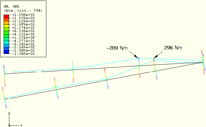
ABAQUS can provide output for structural elements in terms of forces and moments acting on the cross-section at a given point. These section forces and moments are defined in the local beam coordinate system. Contour the section moment about the beam 1-axis in the members of element set OUTA. For clarity, reset the view so that the elements are displayed in the 1–2 plane.
To create a “bending moment”-type contour plot:
From the main menu bar, select Result![]() Field Output.
Field Output.
The Field Output dialog box appears; by default, the Primary Variable tab is selected.
Select SM from the list of available output variables; then select SM1 from the component field.
Click OK.
The Select Plot Mode dialog box appears.
Toggle on Contour, and click OK.
ABAQUS/Viewer displays a contour plot of the bending moment about the beam 1-axis. The contour is plotted on the deformed model shape. The deformation scale factor is chosen automatically since geometric nonlinearity was not considered in the analysis.
Color contour plots of this type typically are not very useful for one-dimensional elements such as beams. A more useful plot is a “bending moment”-type plot, which you can produce using the contour options.
From the prompt area, click Contour Options.
The Contour Plot Options dialog box appears; by default, the Basic tab is selected.
In the Contour Type field, toggle on Show tick marks for line elements.
Click the Shape tab, and select a Uniform deformation scale factor of 1.0.
Click OK.
The plot shown in Figure 6–20 appears. The magnitude of the variable at each node is now indicated by the position at which the contour curve intersects a “tick mark” drawn perpendicular to the element. This “bending moment”-type plot can be used for any variable (not just bending moments) for any one-dimensional element, including trusses and axisymmetric shells as well as beams.