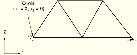
The simulation of the pin-jointed, overhead hoist in Figure 2–1 is used to illustrate the creation of an ABAQUS input file using an editor. As you read through this section, you should type the data into a file using one of the editors available on your computer. The ABAQUS input file must have an .inp file extension. For convenience, name the input file frame.inp. The file identifier, which can be chosen to identify the analysis, is called the jobname. In this case use the jobname “frame” to easily associate it with the input file called frame.inp.
All of the other examples in this guide assume that you will be using a preprocessor, such as ABAQUS/CAE, to generate the mesh if you are going to create the model from scratch. Input files for all the examples are available. See “Execution procedure for ABAQUS/Fetch,” Section 3.2.12 of the ABAQUS Analysis User's Manual, for instructions on how to retrieve these input files. However, since the purpose of this example is to help you understand the structure and format of the ABAQUS input file, you should type this input file in directly, rather than use a preprocessor or copy the input file that is provided. If you wish to create the entire model using ABAQUS/CAE, refer to “Example: creating a model of an overhead hoist with ABAQUS/CAE,” Section 2.3 of Getting Started with ABAQUS.
Before starting to define this or any model, you need to decide which system of units you will use. ABAQUS has no built-in system of units. All input data must be specified in consistent units. Some common systems of consistent units are shown in Table 2–1.
| Quantity | SI | SI (mm) | US Unit (ft) | US Unit (inch) |
|---|---|---|---|---|
| Length | m | mm | ft | in |
| Force | N | N | lbf | lbf |
| Mass | kg | tonne (103 kg) | slug | lbf s2 /in |
| Time | s | s | s | s |
| Stress | Pa (N/m2 ) | MPa (N/mm2 ) | lbf/ft2 | psi (lbf/in2) |
| Energy | J | mJ (10-3 J) | ft lbf | in lbf |
| Density | kg/m3 | tonne/mm3 | slug/ft3 | lbf s2 /in4 |
The SI system of units is used throughout this guide. Users working in the systems labeled “US Unit” should be careful with the units of density; often the densities given in handbooks of material properties are multiplied by the acceleration due to gravity.
You also need to decide which coordinate system to use. The global coordinate system in ABAQUS is a right-handed, rectangular (Cartesian) system. For this example define the global 1-axis to be the horizontal axis of the hoist and the global 2-axis to be the vertical axis (Figure 2–3). The global 3-axis is normal to the plane of the framework. The origin (![]() =0,
=0, ![]() =0,
=0, ![]() =0) is the bottom left-hand corner of the frame.
=0) is the bottom left-hand corner of the frame.
For two-dimensional problems, such as this one, ABAQUS requires that the model lie in a plane parallel to the global 1–2 plane.
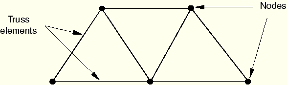
You must select the element types and design the mesh. Creating a proper mesh for a given problem requires experience. For this example you will use a single truss element to model each member of the frame, as shown in Figure 2–4.
A truss element, which can carry only tensile and compressive axial loads, is ideal for modeling pin-jointed frameworks, such as the overhead hoist. Truss elements are described in “Truss elements,” Section 3.1.5, and also in the ABAQUS Analysis User's Manual, which describes every element available in ABAQUS. The index of element types (Section I.1, “ABAQUS/Standard Element Index,” of the ABAQUS Analysis User's Manual) makes locating a particular element easy. Whenever you are using an element for the first time, you should read the description, which includes the element connectivity and any element section properties needed to define the element's geometry.
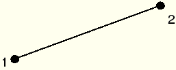
The connectivity for the truss elements used in the overhead hoist model is shown in Figure 2–5.
Node and element numbers are merely identification labels. They are usually generated automatically by ABAQUS/CAE or another preprocessor. The only requirement for node and element numbers is that they must be positive integers. Gaps in the numbering are allowed, and the order in which nodes and elements are defined does not matter. Any nodes that are defined but not associated with an element are removed automatically and are not included in the simulation.
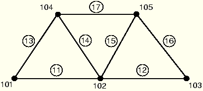
In this case we use the node and element numbers shown in Figure 2–6.
The first part of the input file must contain all of the model data. These data define the structure being analyzed. In the overhead hoist example the model data consist of the following:
Geometry:
Nodal coordinates.
Element connectivity.
Element section properties.
Material properties.
Heading
The first option in any ABAQUS input file must be *HEADING. The data lines that follow the *HEADING option are lines of text describing the problem being simulated. You should provide an accurate description to allow the input file to be identified at a later date. Moreover, it is often helpful to specify the system of units, directions of the global coordinate system, etc. For example, the *HEADING option block for the hoist problem contains the following:
*HEADING
Two-dimensional overhead hoist frame
SI Units
1-axis horizontal, 2-axis vertical
Data file printing options
By default, ABAQUS will not print an echo of the input file or the model and history definition data to the printed output (.dat) file. However, it is recommended that you check your model and history definition in a datacheck run before performing the analysis. The datacheck run is discussed later in this chapter.
To request a printout of the input file and of the model and history definition data, add
*PREPRINT, ECHO=YES, MODEL=YES, HISTORY=YESto the input file.
Nodal coordinates
The coordinates of each node can be defined once you select the mesh design and node numbering scheme. For this problem use the numbering shown in Figure 2–6. The coordinates of nodes are defined using the *NODE option. Each data line of this option block has the form
<node number>,<The nodes for the hoist model are defined as follows:-coordinate>,<
-coordinate>,<
-coordinate>
*NODE
101, 0., 0., 0.
102, 1., 0., 0.
103, 2., 0., 0.
104, 0.5, 0.866, 0.
105, 1.5, 0.866, 0.
Element connectivity
The members of the overhead hoist are modeled with truss elements. The format of each data line for a truss element is
<element number>, <node 1>, <node 2>where node 1 and node 2 are at the ends of the element (see Figure 2–5). For example, element 16 connects nodes 103 and 105 (see Figure 2–6), so the data line defining this element is
16, 103, 105The TYPE parameter on the *ELEMENT option must be used to specify the kind of element being defined. In this case you will use T2D2 truss elements.
One of the most useful features in ABAQUS is the availability of node and element sets that are referred to by name. By using the ELSET parameter on the *ELEMENT option, all of the elements defined in the option block are added to an element set called FRAME. A set name can have as many as 80 characters and must start with a letter. Since element section properties are assigned through element set names, all elements in the model must belong to at least one element set.
The complete *ELEMENT option block for the overhead hoist model (see Figure 2–6) is shown below:
*ELEMENT, TYPE=T2D2, ELSET=FRAME
11, 101,102
12, 102,103
13, 101,104
14, 102,104
15, 102,105
16, 103,105
17, 104,105
Element section properties
Each element must refer to an element section property. The appropriate element section option for each element and the additional geometric data (if any) needed for each element are described in the ABAQUS Analysis User's Manual.
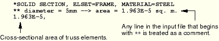
For the T2D2 element you must use the *SOLID SECTION option and give one data line with the cross-sectional area of the element. If you leave the data line blank, the cross-sectional area is assumed to be 1.0.
In this case all the members are circular bars that are 5 mm in diameter. Their cross-sectional area is 1.963 × 10⁻⁵ m2.
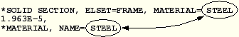
The MATERIAL parameter, which is required for most element section options, refers to the name of a material property definition that is to be used with the elements. The name can have up to 80 characters and must begin with a letter.
In this example all of the elements have the same section properties and are made of the same material. Typically, there will be several different element section properties in an analysis; for example, different components in a model may be made of different materials. The elements are associated with material properties through element sets. For the overhead hoist model the elements are added to an element set called FRAME. Element set FRAME is then used as the value of the ELSET parameter on the element section option. Add the following option block to your input file:
Materials
One of the features that makes ABAQUS a truly general-purpose finite element program is that almost any material model can be used with any element. Once the mesh has been created, material models can be associated, as appropriate, with the elements in the mesh.
ABAQUS has a large number of material models, many of which include nonlinear behavior. In this overhead hoist example we use the simplest form of material behavior: linear elasticity. In Chapter 8, “Materials,” two of the most common forms of nonlinear material behavior are considered: metal plasticity and rubber elasticity. A discussion of all the material models available in ABAQUS/Standard can be found in the ABAQUS Analysis User's Manual.
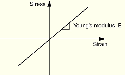
Linear elasticity is appropriate for many materials at small strains, particularly for metals up to their yield point. It is characterized by a linear relationship between stress and strain (Hooke's law), as shown in Figure 2–7.
The material behavior is characterized by two constants: Young's modulus, ![]() , and Poisson's ratio,
, and Poisson's ratio, ![]() .
.
A material definition in the ABAQUS input file starts with a *MATERIAL option. The parameter NAME is used to associate a material with an element section property. For example,
Material suboptions directly follow their associated *MATERIAL option. Several suboptions may be required to complete the material definition. All material suboptions are associated with the material that is listed on the most recent *MATERIAL option until another *MATERIAL option or a non-material option block is given.
Without considering thermal expansion effects (which would be defined with the *EXPANSION material suboption), one material suboption, *ELASTIC, is required to define a linear elastic material. The form of this option block is
*ELASTIC <E>,<Therefore, the complete, isotropic, linear elastic material definition for the hoist members, which are made of steel, should be entered into your input file as>
*MATERIAL, NAME=STEEL
*ELASTIC
200.E9, 0.3
The model definition portion of this problem is now complete since all the components describing the structure have been specified.
The history data define the sequence of events for the simulation. This loading history is divided into a series of steps, each defining a different portion of the structure's loading. Each step contains the following information:
the type of simulation (static, dynamic, etc.);
the loads and constraints; and
the output required.
In this example we are interested in the static response of the overhead hoist to a 10 kN load applied at the center, with the left-hand end fully constrained and a roller constraint on the right-hand end (see Figure 2–1). This is a single event, so only a single step is needed for the simulation.
The *STEP option is used to mark the start of a step. Like the *HEADING option, this option may be followed by data lines containing a title for the step. In your hoist model use the following *STEP option block:
*STEP,PERTURBATION
10kN central load
The PERTURBATION parameter indicates that this is a linear analysis. If this parameter is omitted, the analysis may be linear or nonlinear. The use of the PERTURBATION parameter is discussed further in Chapter 10, “Multiple Step Analysis.”
Analysis procedure
The analysis procedure (the type of simulation) must be defined immediately following the *STEP option block. In this case we want the long-term static response of the structure. The option for a static simulation is *STATIC. For linear analysis this option has no parameters or data lines, so add the following line to your input file:
*STATIC
The remaining input data in the step define the boundary conditions (constraints), loads, and output required and can be given in any order that is convenient.
Boundary conditions
Boundary conditions are applied to those parts of the model where the displacements are known. Such parts may be constrained to remain fixed (have zero displacement) during the simulation or may have specified, nonzero displacements. In either situation the constraints are applied directly to the nodes of the model.
In some cases a node may be constrained completely and, thus, cannot move in any direction (for example, node 101 in our case). In other cases a node is constrained in some directions but is free to move in others. For example, node 103 is fixed in the vertical direction but is free to move in the horizontal direction. The directions in which a node is able to move are called degrees of freedom (dof). In the case of our two-dimensional hoist, each node can move in the global 1- and 2-directions; therefore, there are two degrees of freedom at each node. If the hoist could move out of plane, the problem would be three-dimensional, and each node would have three degrees of freedom. Nodes attached to beam and shell elements have additional degrees of freedom representing the components of rotation and, thus, may have up to six degrees of freedom.
The labeling convention used for the degrees of freedom in ABAQUS is as follows:

The degrees of freedom active at a node depend on the type of elements attached to that node. Chapter 3, “Finite Elements and Rigid Bodies,” describes the active degrees of freedom for some of the elements available in ABAQUS. The two-dimensional truss element, T2D2, has two degrees of freedom active at each node—translation in the 1- and 2-directions (dof 1 and dof 2).
Constraints on nodes are defined by using the *BOUNDARY option and specifying the constrained degrees of freedom. Each data line is of the form:
<node number>, <first dof>, <last dof>, <magnitude of displacement>
The first degree of freedom and last degree of freedom are used to give a range of degrees of freedom that will be constrained. For example,
101, 1, 3, 0.0constrains degrees of freedom 1, 2, and 3 at node 101 to have zero displacement (the node cannot move in either the global 1-, 2-, or 3-direction).
If the magnitude of the displacement is not specified on the data line, it is assumed to be zero. If the node is constrained in one direction only, the third field should be blank or equal to the second field. For example, to constrain node 103 in the 2-direction (degree of freedom 2) only, any of the following data line formats can be used:
103, 2,2, 0.0or
103, 2,2or
103, 2
Boundary conditions on a node are cumulative. Thus, the following input constrains node 101 in both directions 1 and 2:
101, 1
101, 2
Rather than specifying each constrained degree of freedom, some of the more common constraints can be given directly using the following named constraints:
| ENCASTRE | Constraint on all displacements and rotations at a node. |
| PINNED | Constraint on all translational degrees of freedom. |
| XSYMM | Symmetry constraint about a plane of constant |
| YSYMM | Symmetry constraint about a plane of constant |
| ZSYMM | Symmetry constraint about a plane of constant |
| XASYMM | Antisymmetry constraint about a plane of constant |
| YASYMM | Antisymmetry constraint about a plane of constant |
| ZASYMM | Antisymmetry constraint about a plane of constant |
101, ENCASTRE
The complete *BOUNDARY option block for our hoist problem is:
*BOUNDARY
101,ENCASTRE
103,2
In this example all of the constraints are in the global 1- or 2-directions. In many cases constraints are required in directions that are not aligned with the global directions. The *TRANSFORM option can be used in such cases to define a local coordinate system for boundary condition application. The skew plate example in Chapter 5, “Using Shell Elements,” demonstrates how to use this option in such cases.
Loading
Loading is anything that causes the displacement or deformation of the structure, including:
concentrated loads,
pressure loads,
distributed traction loads,
distributed edge loads and moment on shells,
nonzero boundary conditions,
body loads, and
temperature (with thermal expansion of the material defined).
In reality there is no such thing as a concentrated, or point, load; the load will always be applied over some finite area. However, if the area being loaded is similar to or smaller than the elements in that area, it is an appropriate idealization to treat the load as a concentrated load applied to a node.
Concentrated loads are specified using the *CLOAD option. The data lines for this option have the form:
<node number>, <dof>, <load magnitude>In this simulation a load of –10 kN is applied in the 2-direction to node 102. The option block is:
*CLOAD
102, 2, -10.E3
Output requests
Finite element analyses can create very large amounts of output. ABAQUS allows you to control and manage this output so that only data required to interpret the results of your simulation are produced. Four types of output are available:
Results stored in a neutral binary file used by ABAQUS/Viewer for postprocessing. This file is called the ABAQUS output database file and has the extension .odb.
Printed tables of results, written to the ABAQUS data (.dat) file.
Restart data, used to continue the analysis, written to the ABAQUS restart (.res) file.
Results stored in binary files for subsequent postprocessing with third-party software, written to the ABAQUS results (.fil) file.
By default, an output database file, which includes a preselected set of the most commonly used output variables for a given type of analysis, is created. A list of preselected variables for default output database output is given in the ABAQUS Analysis User's Manual. You do not need to add any output requests to accept these defaults. For this example the default output database output includes the deformed configuration and the applied nodal loads.
Selected results also can be written in tabular form to the ABAQUS data file. By default, no printout is written to the ABAQUS data file. The *NODE PRINT option controls the printing of nodal results (for example, displacements and reaction forces), while the *EL PRINT option controls the printing of element results. A comprehensive list of the output variables available is given in the ABAQUS Analysis User's Manual.
The data lines for either of these options list the output to appear in the columns of the table. Each data line creates a separate table of data that can have a maximum of nine columns.
For this analysis we are interested in the displacements of the nodes (output variable U), the reaction forces at the constrained nodes (output variable RF), and the stress in the members (output variable S). Use the following in your input file:
*NODE PRINT
U,
RF,
*EL PRINT
S,
to request that ABAQUS generate three tables of output data in the data file.
Since you have now finished the definition of all the data required for the step, use the *END STEP option to mark the end of the step:
*END STEP
The input file is now complete. Compare the input file you have generated to the complete input file given in Figure 2–2. Save the data as frame.inp, and exit the editor.