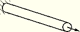
This section reviews the basics of the finite element method. A simple example of a truss, constrained at one end and loaded at the other end as shown in Figure 1–2, is used to introduce some terms and conventions used in the rest of this document. The objective of the analysis is to find the displacement of the free end of the truss, the stress in the truss, and the reaction force at the constrained end of the truss.

The first step of any finite element simulation is to discretize the actual geometry of the structure using a collection of finite elements. Each finite element represents a discrete portion of the physical structure. The finite elements are joined by shared nodes.The collection of nodes and finite elements is called the mesh. The number of elements used in a particular mesh is referred to as the mesh density. In a stress analysis the displacements of the nodes are the fundamental variables that ABAQUS calculates. Once the nodal displacements are known, the stresses and strains in each finite element can be determined easily.

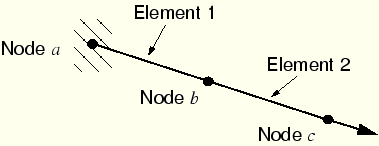
In this case the rod shown in Figure 1–2 will be modeled with two truss elements. In ABAQUS truss elements can carry axial loads only. The discretized model is shown in Figure 1–3 together with the node and element labels.

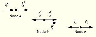
Free-body diagrams for each node in the model are shown in Figure 1–4. In general each node will carry an external load applied to the model, , and internal loads, , caused by stresses in the elements attached to that node. For a model to be in static equilibrium, the net force acting on each node must be zero; i.e., the internal and external loads at each node must balance each other. For node this equilibrium equation can be obtained as follows.

Assuming that the change in length of the rod is small, the strain in element 1 is given by

where and are the displacements at nodes and , respectively, and is the original length of the element.

Assuming that the material is elastic, the stress in the rod is given by the strain multiplied by the Young's modulus, :

The axial force acting on the end node is equivalent to the stress in the rod multiplied by its cross-sectional area, . Thus, a relationship between internal force, material properties, and displacements is obtained:

Equilibrium at node can, therefore, be written as

Equilibrium at node must take into account the internal forces acting from both elements joined at that node. The internal force from element 1 is now acting in the opposite direction and so becomes negative. The resulting equation is

For node c the equilibrium equation is

These equilibrium equations need to be solved simultaneously to obtain the displacements of all the nodes. This requirement is best achieved by matrix techniques; therefore, write the internal and external force contributions as matrices. If the properties and dimensions of the two elements are the same, the equilibrium equations can be simplified as follows:

In general, it may be that the element stiffnesses, the terms, are different from element to element; therefore, write the element stiffnesses as and for the two elements in the model. We are interested in obtaining the solution to the equilibrium equation in which the externally applied forces, , are in equilibrium with the internally generated forces, . When discussing this equation with reference to convergence and nonlinearity, we write it as

For the complete two-element, three-node structure we, therefore, modify the signs and rewrite the equilibrium equation as

This system of equations can then be solved to obtain values for the three unknown variables: , , and ( is specified in the problem as 0.0). Once the displacements are known, we can go back and use them to calculate the stresses in the truss elements.