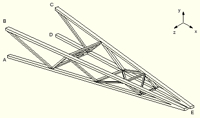
This example uses the same cargo crane that you analyzed in “Example: cargo crane,” Section 6.4, but you have now been asked to investigate what happens when a load of 10 kN is dropped onto the lifting hook for 0.2 seconds. The connections at points A, B, C, and D (see Figure 7–5) can only withstand a maximum pull-out force of 100 kN. You have to decide whether or not any of these connections will break.
The short duration of the loading means that inertia effects are likely to be important, making dynamic analysis essential. You are not given any information regarding the damping of the structure. Since there are bolted connections between the trusses and the cross bracing, the energy absorption caused by frictional effects is likely to be significant. Based on experience, you therefore choose 5% of critical damping in each mode.
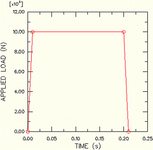
The magnitude of the applied load versus time is shown in Figure 7–6.
A Python script is provided in “Cargo crane – dynamic loading,” Section A.5. When this script is run through ABAQUS/CAE, it creates the complete analysis model for this problem. Run this script if you encounter difficulties following the instructions given below or if you wish to check your work. Instructions on how to fetch and run the script are given in Appendix A, “Example Files.”
If you do not have access to ABAQUS/CAE or another preprocessor, the input file required for this problem can be created manually, as discussed in “Example: cargo cranedynamic loading,” Section 9.5 of Getting Started with ABAQUS/Standard: Keywords Version.
Open the model database file Crane.cae, and copy the Static model to a model named Dynamic. The dynamic analysis model is basically the same as the static analysis model, except for the modifications described below.
Material
In dynamic simulations the density of every material must be specified so that the mass matrix can be formed. The steel in the crane has a density of 7800 kg/m3.
In this model the material properties were specified as part of the section definition. Thus, you will need to edit the BracingSection and MainMemberSection section definitions to specify the density. In the Section material density field of the Edit Beam Section dialog box, enter a value of 7800 for each section definition.
Note:
If material data are defined independently of the section properties, the density is included by editing the material definition and selecting General![]() Density in the Edit Material dialog box.
Density in the Edit Material dialog box.
Steps
The step definitions that are used for the dynamic analysis are substantially different from those used in the static analysis. Therefore, the static step created previously will be replaced by two new steps.
The first step in the dynamic analysis calculates the natural frequencies and mode shapes of the structure. The second step then uses these data to calculate the transient (modal) dynamic response of the hoist. In this analysis we will assume that everything is linear. If you want to model any nonlinearities in this simulation, direct integration of the equations of motion using the implicit dynamic procedure must be performed instead. See “Nonlinear dynamics,” Section 7.9.2, for further details.
ABAQUS/Standard offers the Lanczos and the subspace iteration eigenvalue extraction methods. The Lanczos method is generally faster when a large number of eigenmodes is required for a system with many degrees of freedom. The subspace iteration method may be faster when only a few (less than 20) eigenmodes are needed.
We use the Lanczos eigensolver in this analysis and request the first 30 eigenvalues. Instead of specifying the number of modes required, it is also possible to specify the minimum and maximum frequencies of interest so that the step will complete once ABAQUS/Standard has found all of the eigenvalues inside the specified range. A shift point may also be specified so that eigenvalues nearest the shift point will be extracted. By default, no minimum or maximum frequency or shift is used. If the structure is not constrained against rigid body modes, the shift value should be set to a small negative value to remove numerical problems associated with rigid body motion.
To replace the static step with a frequency extraction step:
In the Model Tree, expand the Steps container. Then, click mouse button 3 on the step named Tip Load and select Replace from the menu that appears. In the Replace Step dialog box, select Frequency from the list of available Linear perturbation procedures.
Model attributes that cannot be converted will be deleted. In this case the concentrated loads are deleted because they cannot be used in a frequency extraction step. However, the boundary conditions and output requests associated with the static step are inherited by the frequency extraction step.
In the Basic tabbed page of the Edit Step dialog box, enter the step description First 30 modes; accept the Lanczos eigensolver option; and request the first 30 eigenvalues.
Rename the step to Extract Frequencies.
In structural dynamic analysis the response is usually associated with the lower modes. However, enough modes should be extracted to provide a good representation of the dynamic response of the structure. One way of checking that a sufficient number of eigenvalues has been extracted is to look at the total effective mass in each degree of freedom, which indicates how much of the mass is active in each direction of the extracted modes. The effective masses are tabulated in the data file under the eigenvalue output. Ideally, the sum of the modal effective masses for each mode in each direction should be at least 90% of the total mass. This is discussed further in “Effect of the number of modes,” Section 7.6.
The modal dynamics procedure will be used to perform the transient dynamic analysis. The transient response will be based on all the modes extracted in the first analysis step; 5% of critical damping should be used in all 30 modes.
To create a transient modal dynamics step:
In the Model Tree, double-click the Steps container to create a new step. Select Modal dynamics from the list of available Linear perturbation procedures, and name the step Transient modal dynamics. Insert the step after the frequency extraction step defined above.
In the Basic tabbed page of the Edit Step dialog box, enter the description Simulation of Load Dropped on Crane and specify a time period of 0.5 and a time increment of 0.005. In dynamic analysis time is a real, physical quantity.
In the Damping tabbed page of the Edit Step dialog box, specify direct modal damping and enter a critical damping fraction of 0.05 for modes 1 through 30.
The eigenmodes used in a mode-based dynamic procedure must be specified if modal damping is used. By default, ABAQUS/CAE automatically selects all available eigenmodes. You may use the Keywords Editor, however, to edit the *SELECT EIGENMODES block if you wish to change the default selection. In this problem, accept the default selection.
Output
Using the Field Output Requests Manager, modify the field output requests for the Extract Frequencies step so that the Preselected defaults are selected. By default, ABAQUS/Standard writes the mode shapes to the output database (.odb) file so that they can be plotted using the Visualization module. The nodal displacements for each mode shape are normalized so that the maximum displacement is unity. Thus, these results, and the corresponding stresses and strains, are not physically meaningful: they should be used only for relative comparisons.
Dynamic analyses usually require many more increments than static analyses to complete. As a consequence, the volume of output from dynamic analyses can be very large, and you should control the output requests to keep the output files to a reasonable size. In this example you will request output of the deformed shape to the output database file at the end of every fifth increment. There will be 100 increments in the step (0.5/0.005); therefore, there will be 20 frames of field output.
In addition, you will write the displacements at the loaded end of the model (for example, set Tip-a) and the reaction forces at the fixed end (set Attach) as history data to the output database file every increment so that a higher resolution of these data will be available. In dynamic analyses we are also concerned about the energy distribution in the model and what form the energy takes. Kinetic energy is present in the model as a result of the motion of the mass; strain energy is present as a result of the displacement of the structure; energy is also dissipated through damping. By default, whole model energies are written as history data to the .odb file for the modal dynamics procedure.
To request output for the transient modal dynamics analysis step:
Open the Field Output Requests Manager. Select the cell labeled Created that appears in the column labeled Transient modal dynamics (you may need to enlarge the column to see the complete step name).
Edit the field output request so that only the nodal displacements are written to the .odb file every 5 increments.
Open the History Output Requests Manager. Create two new output requests in the step labeled Transient modal dynamics. In the first write the displacements for the set Tip-a after every increment; in the second, the reaction forces for the set Attach after every increment.
Loads and boundary conditions
The boundary conditions are the same as for the static analysis. Since these were retained during the step replacement operation, no new boundary conditions need to be defined.
Apply a concentrated point load to the tip of the crane. The magnitude of this concentrated load is time dependent, as illustrated in Figure 7–6. The time dependence of the load can be defined using an amplitude curve. The actual magnitude of the load applied at any point in time is obtained by multiplying the magnitude of the load (–10,000 N) by the value of the amplitude curve at that time.
To specify a time-dependent load:
Begin by defining an amplitude. In the Model Tree, double-click the Amplitudes container. Name the amplitude Bounce, and choose the type Tabular. Enter the data shown in Table 7–1 in the Edit Amplitude dialog box. Accept the default selection of Step time as the time span, and specify 0.25 as the smoothing parameter value.
Tip: Use mouse button 3 to access the table options.
Now define the load. In the Model Tree, double-click the Loads container. Apply the load in the Transient modal dynamics step, name the load Tip load, and choose Concentrated force as the load type. Apply the load to set Tip-b. The equation constraint defined previously between sets Tip-a and Tip-b means that the load will be carried equally by both halves of the crane.
In the Edit Load dialog box, enter a value for CF2 of -1.E4, and choose Bounce for the amplitude.
In this example the structure has no initial velocities or accelerations, which is the default. However, if you wanted to define initial velocities, you could do so by selecting Field![]() Create from the main menu bar and assigning initial translational velocities to selected regions of the model in the initial step. You would also have to edit the definition of the modal dynamics step to use initial conditions.
Create from the main menu bar and assigning initial translational velocities to selected regions of the model in the initial step. You would also have to edit the definition of the modal dynamics step to use initial conditions.
Running the analysis
Create a job named DynCrane with the following description: 3-D model of light-service cargo crane dynamic analysis.
Save your model in a model database file, and submit the job for analysis. Monitor the solution progress; correct any modeling errors that are detected and investigate the cause of any warning messages, taking action as necessary.
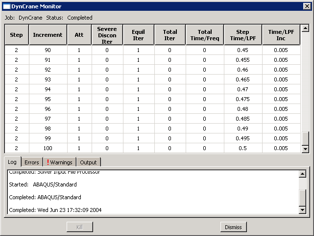
The Job Monitor gives a brief summary of the automatic time incrementation used in the analysis for each increment. The information is written as soon as the increment is completed, so that you can monitor the analysis as it is running. This facility is useful in large, complex problems. The information given in the Job Monitor is the same as that given in the status file (DynCrane.sta).
Examine the Job Monitor and the printed output data file (DynCrane.dat) to evaluate the analysis results.
Job monitor
In the Job Monitor, the first column shows the step number and the second column gives the increment number. The sixth column shows the number of iterations ABAQUS/Standard needed to obtain a converged solution in each increment. Looking at the contents of the Job Monitor, we can see that the time increment associated with the single increment in Step 1 is very small. This step uses no time, because time is not relevant in a frequency extraction procedure.
The output for Step 2 shows that the time increment size is constant throughout the step and that each increment requires only one iteration. The bottom of the Job Monitor is shown in Figure 7–7.
Data file
The primary results for Step 1 are the extracted eigenvalues, participation factors, and effective mass, as shown below.
E I G E N V A L U E O U T P U T
MODE NO EIGENVALUE FREQUENCY GENERALIZED MASS COMPOSITE MODAL DAMPING
(RAD/TIME) (CYCLES/TIME)
1 1773.5 42.113 6.7025 151.93 0.0000
2 7016.2 83.763 13.331 30.208 0.0000
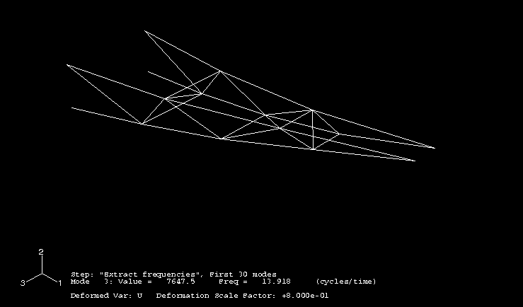
3 7647.5 87.450 13.918 90.342 0.0000
4 22990. 151.62 24.132 251.91 0.0000
5 24702. 157.17 25.014 273.76 0.0000
6 34722. 186.34 29.656 487.55 0.0000
7 42846. 206.99 32.944 1133.2 0.0000
8 46446. 215.51 34.300 86.044 0.0000
9 47424. 217.77 34.659 2549.7 0.0000
10 56035. 236.72 37.675 3573.6 0.0000
....
25 2.25734E+05 475.11 75.617 202.15 0.0000
26 2.42424E+05 492.37 78.362 126.39 0.0000
27 2.84031E+05 532.95 84.821 1254.6 0.0000
28 2.92366E+05 540.71 86.056 336.51 0.0000
29 3.13942E+05 560.31 89.175 272.82 0.0000
30 3.64671E+05 603.88 96.110 65.354 0.0000The highest frequency extracted is 96 Hz. The period associated with this frequency is 0.0104 seconds, which is comparable to the fixed time increment of 0.005 seconds. There is no point in extracting modes whose period is substantially smaller than the time increment used. Conversely, the time increment must be capable of resolving the highest frequencies of interest.The column for generalized mass lists the mass of a single degree of freedom system associated with that mode.
The table of participation factors indicates the predominant degrees of freedom in which the modes act. The results indicate, for example, that mode 1 acts predominantly in the 3-direction.
          P A R T I C I P A T I O N   F A C T O R S

 MODE NO    X-COMPONENT    Y-COMPONENT    Z-COMPONENT    X-ROTATION     Y-ROTATION     Z-ROTATION

       1     -6.07366E-04   -6.17116E-03     1.4284        0.71334        -6.0252       -3.38295E-02
       2      0.18478       -0.25741        8.07283E-04    1.70643E-03   -6.15528E-03    -1.6861
       3     -0.17450         1.5525        4.87105E-03   -8.03502E-03    3.24238E-02     9.2789
       4     -1.15540E-04   -9.14309E-03    8.21369E-02    0.21835         1.2228       -2.82698E-02
       5     -3.92365E-03    2.10839E-03   -3.00589E-02   -0.59334         1.7705       -1.93065E-02
       6      3.71444E-02   -0.35739        6.34646E-03   -1.76999E-02    9.99848E-03   -0.96547
       7     -2.48995E-03   -1.51233E-03    6.05075E-02    4.76131E-02   -0.29185       -5.86262E-04
       8     -7.05056E-02    2.47060E-02    0.72588        0.49699        -3.8837        7.04118E-02
       9      3.61761E-02   -2.42235E-02    2.25532E-02    1.50086E-02   -0.12937       -9.47618E-04
      10      3.47956E-02    4.06055E-02    1.95085E-02    1.09153E-02   -6.75409E-02    3.81548E-02
....
      25     -8.03494E-02   -0.20584       -3.85110E-02    4.64402E-02   -2.61035E-02   -0.17918
      26     -2.46693E-02   -0.36460        4.43708E-02   -2.04556E-02   -1.17708E-02   -0.19900
      27      1.69765E-02    2.49820E-02    2.25071E-02   -1.01230E-02   -4.29483E-02    2.77695E-02
      28      4.67016E-02    2.75667E-02   -0.11801        5.13385E-02    0.24067        2.78739E-05
      29      9.82729E-03   -3.65328E-03    4.60058E-03   -3.12278E-03   -1.55601E-02   -2.79285E-03
      30      4.78413E-02    1.80146E-02    0.13095       -2.16793E-02   -0.34987       -1.79423E-02
The table of effective mass indicates the amount of mass active in each degree of freedom for any one mode. The results indicate that the first mode with significant mass in the 2-direction is mode 3. The total modal effective mass is 378.25 kg. E F F E C T I V E M A S S
MODE NO X-COMPONENT Y-COMPONENT Z-COMPONENT X-ROTATION Y-ROTATION Z-ROTATION
1 5.60455E-05 5.78593E-03 309.98 77.308 5515.4 0.17387
2 1.0314 2.0016 1.96869E-05 8.79633E-05 1.14452E-03 85.883
3 2.7508 217.75 2.14356E-03 5.83262E-03 9.49771E-02 7778.3
4 3.36289E-06 2.10587E-02 1.6995 12.010 376.67 0.20132
5 4.21453E-03 1.21694E-03 0.24735 96.379 858.18 0.10204
6 0.67268 62.272 1.96374E-02 0.15274 4.87405E-02 454.46
7 7.02540E-03 2.59168E-03 4.1487 2.5689 96.521 3.89469E-04
8 0.42773 5.25199E-02 45.337 21.253 1297.8 0.42659
9 3.3369 1.4961 1.2969 0.57435 42.676 2.28960E-03
10 4.3267 5.8922 1.3601 0.42578 16.302 5.2025
....
25 1.3051 8.5651 0.29981 0.43598 0.13774 6.4899
26 7.69154E-02 16.801 0.24883 5.28843E-02 1.75110E-02 5.0050
27 0.36158 0.78300 0.63554 0.12856 2.3142 0.96747
28 0.73394 0.25572 4.6865 0.88692 19.492 2.61453E-07
29 2.63481E-02 3.64123E-03 5.77439E-03 2.66050E-03 6.60551E-02 2.12803E-03
30 0.14958 2.12093E-02 1.1206 3.07161E-02 7.9998 2.10393E-02
TOTAL 22.181 378.25 373.63 269.75 8348.0 8518.0The total mass of the model is given earlier in the data file and is 414.34 kg.To ensure that enough modes have been used, the total effective mass in each direction should be a large proportion of the mass of the model (say 90%). However, some of the mass of the model is associated with nodes that are constrained. This constrained mass is approximately one-quarter of the mass of all the elements attached to the constrained nodes, which, in this case, is approximately 28 kg. Therefore, the mass of the model that is able to move is 385 kg. The effective mass in the x-, y-, and z-directions is 6%, 98%, and 97%, respectively, of the mass that can move. The total effective mass in the 2- and 3-directions is well above the 90% recommended earlier; the total effective mass in the 1-direction is much lower. However, since the loading is applied in the 2-direction, the response in the 1-direction is not significant.
The data file does not contain any results for the modal dynamics step, because all of the data file output requests were suppressed.
Enter the Visualization module, and open the output database file DynCrane.odb.
Plotting mode shapes
You can visualize the deformation mode associated with a given natural frequency by plotting the mode shape associated with that frequency.
To select a mode and plot the corresponding mode shape:
From the main menu bar, select Result![]() Step/Frame.
Step/Frame.
The Step/Frame dialog box appears.
Select the first step (Extract Frequencies) from the Step Name list.
Select Mode 1 from the Frame list.
From the main menu bar, select Plot![]() Deformed Shape; or use the
Deformed Shape; or use the ![]() tool in the toolbox.
tool in the toolbox.
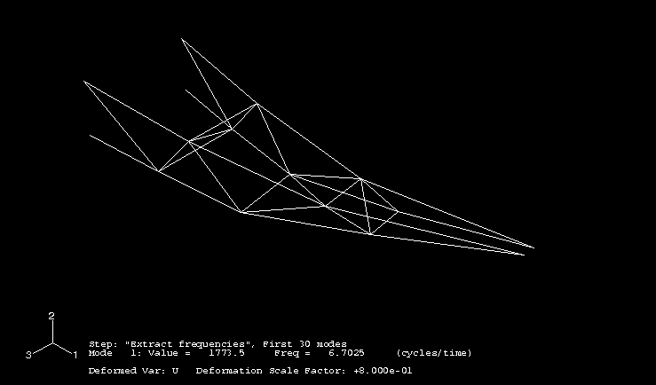
ABAQUS/CAE displays the deformed model shape associated with the first vibration mode, as shown in Figure 7–8.
Select the third mode from the Step/Frame dialog box.
Click OK.
ABAQUS/CAE displays the third mode shape shown in Figure 7–9, and the Step/Frame dialog box disappears.
Animation of results
You will animate the analysis results. First create a scale factor animation of the third eigenmode. Then create a time-history animation of the transient results.
To create a scale factor animation of an eigenmode:
From the main menu bar, select Animate![]() Scale Factor; or use the
Scale Factor; or use the ![]() tool in the toolbox.
tool in the toolbox.
ABAQUS/CAE displays the third mode shape and steps through different deformation scale factors ranging from 0 to 1.
ABAQUS/CAE also displays the movie player controls on the left side of the prompt area.
In the prompt area, click ![]() to stop the animation.
to stop the animation.
To create a time-history animation of the transient results:
From the main menu bar, select Options![]() Animation to view the animation options.
Animation to view the animation options.
ABAQUS/CAE displays the Animation Options dialog box.
Click the Time History tab.
Select the second step (Transient modal dynamics).
Click OK to accept the selection and to close the dialog box.
From the main menu bar, select Animate![]() Time History; or use the
Time History; or use the ![]() tool from the toolbox.
tool from the toolbox.
ABAQUS/CAE displays the movie player controls on the left side of the prompt area and steps through each available frame of the second step. The state block indicates the current step and increment throughout the animation. After the last increment of this step is reached, the animation process repeats itself.
You can customize the deformed shape plot while the animation is running.
Display the Deformed Shape Plot Options dialog box.
Choose Uniform from the Deformation Scale Factor field.
Enter 15.0 as the deformation scale factor value.
Click Apply to apply your change.
ABAQUS/CAE now steps through the frames in the second step with a deformation scale factor of 15.0.
Choose Auto-compute from the Deformation Scale Factor field.
Click OK to apply your change and to close the Deformed Shape Plot Options dialog box.
ABAQUS/CAE now steps through the frames in the second step with a default deformation scale factor of 0.8.
Determining the peak pull-out force
To find the peak pull-out force at the attachment points, create an X–Y plot of the reaction force in the 1-direction (variable RF1) at the attached nodes. This involves plotting multiple curves at the same time.
To plot multiple curves:
From the main menu bar, select Result![]() History Output.
History Output.
ABAQUS/CAE displays the History Output dialog box.
From the Output Variables field on the Variables tabbed page, select the four curves (using [Ctrl]+Click) that have the following form:
Reaction Force: RF1 PI: TRUSS-1 Node xxx in NSET ATTACH
Click Plot.
ABAQUS/CAE displays the selected curves.
From the main menu bar, select Viewport![]() Viewport Annotation Options.
Viewport Annotation Options.
ABAQUS/CAE displays the Viewport Annotation Options dialog box.
Click the Legend tab, and toggle on Show min/max values.
Click OK to apply your change and to close the dialog box.
ABAQUS/CAE displays the minimum and maximum values.
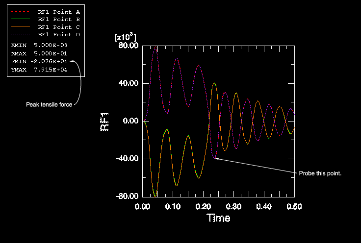
The resulting plot (which has been customized) is shown in Figure 7–10. The curves for the two nodes at the top of each truss (points B and C) are almost a reflection of those for the nodes on the bottom of each truss (points A and D).
At the attachment points at the top of each truss structure, the peak tensile force is around 80 kN, which is below the 100 kN capacity of the connection. Keep in mind that a negative reaction force in the 1-direction means that the member is being pulled away from the wall. The lower attachments are in compression (positive reaction force) while the load is applied, but oscillate between tension and compression after the load has been removed. The peak tensile force is about 40 kN, well below the allowable value. To find this value, probe the X–Y plot.
To query the X–Y plot:
From the main menu bar, select Tools![]() Query.
Query.
The Query dialog box appears.
Select Probe values in the Visualization Queries field.
Click OK.
The Probe Values dialog box appears.
Select the point indicated in Figure 7–10.
The ![]() -coordinate of this point is –40.3 kN, which corresponds to the value of the reaction force in the 1-direction.
-coordinate of this point is –40.3 kN, which corresponds to the value of the reaction force in the 1-direction.