You use the Visualization module to read the output database that ABAQUS/CAE generated during the analysis and to view the results of the analysis. Because you named the job Deform when you created the job, ABAQUS/CAE names the output database Deform.odb.
When you open an output database, ABAQUS/CAE immediately displays a fast representation of the model that is similar to an undeformed shape plot. For the tutorial you will also view an undeformed, deformed, and contour plot of the loaded cantilever beam.
To view the results of your analysis:
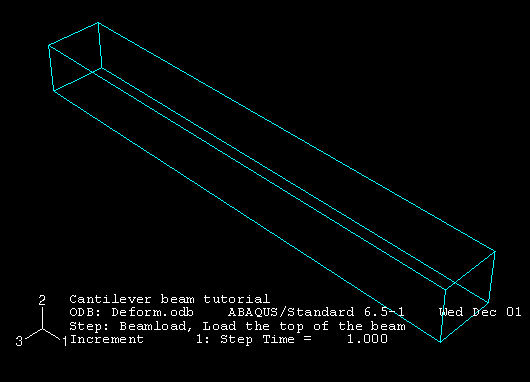
After you select Results in the Model Tree, ABAQUS/CAE enters the Visualization module, opens Deform.odb, and displays a fast plot of the model, as shown in Figure B–13.
The title block indicates the following:The job description.
The output database from which ABAQUS/CAE read the data.
The version of ABAQUS/Standard or ABAQUS/Explicit that was used to generate the output database.
The date the output database was generated.
The step name and the step description.
The increment within the step.
The step time.
When you are viewing a deformed plot, the deformed variable and the deformation scale factor.
From the main menu bar, select Plot![]() Undeformed Shape to view an undeformed shape plot.
Undeformed Shape to view an undeformed shape plot.
The model's color changes to green to indicate that this is an undeformed shape plot, not a fast plot.
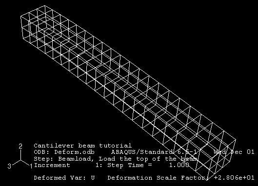
From the main menu bar, select Plot![]() Deformed Shape to view a deformed shape plot.
Deformed Shape to view a deformed shape plot.
Click the auto-fit tool ![]() so that the entire plot is rescaled to fit in the viewport, as shown in Figure B–14.
so that the entire plot is rescaled to fit in the viewport, as shown in Figure B–14.
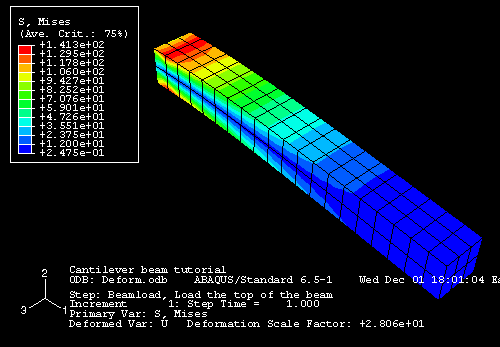
From the main menu bar, select Plot![]() Contours to view a contour plot of the von Mises stress, as shown in Figure B–15.
Contours to view a contour plot of the von Mises stress, as shown in Figure B–15.
Click the Contour Options button at the bottom-right corner of the prompt area to change the appearance of the current plot.
The Contour Plot Options dialog box appears. You can use this dialog box to, for example, turn on node and element labeling, change the deformation scale factor of the underlying model, or adjust the contour intervals. (To change general plot options, such as turning the legend off or on, select Viewport![]() Viewport Annotation Options from the main menu bar.)
Viewport Annotation Options from the main menu bar.)
Click Cancel to close the Contour Plot Options dialog box.
For a contour plot the default variable displayed depends on the analysis procedure; in this case, the default variable is the von Mises stress. From the main menu bar, select Result![]() Field Output to examine the variables that are available for display.
Field Output to examine the variables that are available for display.
ABAQUS/CAE displays the Field Output dialog box; click the Primary Variable tab to choose which variable to display and to select the invariant or component of interest. By default, the Mises invariant of the Stress components at integration points variable is selected.
Click Cancel to close the Field Output dialog box.
You have now finished this tutorial. Appendix C, “Using Additional Techniques to Create and Analyze a Model in ABAQUS/CAE,” introduces additional techniques to create and analyze a model; for example, you will create and assemble multiple part instances and define contact. Appendix D, “Viewing the Output from Your Analysis,” covers the capabilities of the Visualization module in more detail.
For information on related topics, click any of the following items: