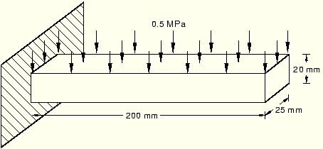
This example uses ABAQUS Scripting Interface commands to reproduce the cantilever beam tutorial described in Appendix B, “Creating and Analyzing a Simple Model in ABAQUS/CAE,” of Getting Started with ABAQUS. Figure 7–1 illustrates the model that you will create and analyze.
The following topics are covered:Use the following command to retrieve the output database that is read by the scripts:
abaqus fetch job=beamExample
To run the script, do the following:
Start ABAQUS/CAE from a directory in which you have write permission by typing abaqus cae.
From the startup screen, select Run Script.
From the Run Script dialog box that appears, enter the path given above and select the file containing the script.
Click OK to run the script.
Note:
If ABAQUS/CAE is already running, you can run the script by selecting File![]() Run Script from the main menu bar.
Run Script from the main menu bar.
The first line of the script, from abaqus import *, imports the Mdb and Session objects. The current viewport is session.viewports['Viewport: 1'], and the current model is mdb.models['Model-1']. Both of these objects are available to the script after you import the abaqus module. The second line of the script, from abaqusConstants import *, imports the Symbolic Constants defined in the ABAQUS Scripting Interface. The script then creates a new model that will contain the cantilever beam example and creates a new viewport in which to display the model and the results of the analysis. For a description of the commands used in this section, see the appropriate sections in the ABAQUS Scripting Reference Manual.
The script then imports the Part module. Most of the sections in this example begin with importing the appropriate module, which illustrates how a script can import a module at any time to extend or augment the object model. However, the ABAQUS Scripting Interface has a convention that all the required modules are imported at the start of a script; and that convention is followed in other example scripts in this manual.
"""
beamExample.py

Reproduce the cantilever beam example from the
Appendix of the Getting Started with
ABAQUS Manual.
"""

from abaqus import *
from abaqusConstants import *

# Create a model.

myModel = mdb.Model(name='Beam')

# Create a new viewport in which to display the model
# and the results of the analysis.

myViewport = session.Viewport(name='Cantilever Beam Example',
    origin=(20, 20), width=150, height=120)

#-----------------------------------------------------

import part

# Create a sketch for the base feature.

mySketch = myModel.Sketch(name='beamProfile',
    sheetSize=250.)

# Create the rectangle.

mySketch.rectangle(point1=(-100,10), point2=(100,-10))

# Create a three-dimensional, deformable part.

myBeam = myModel.Part(name='Beam', dimensionality=THREE_D,
    type=DEFORMABLE_BODY)

# Create the part's base feature by extruding the sketch
# through a distance of 25.0.

myBeam.BaseSolidExtrude(sketch=mySketch, depth=25.0)

#-----------------------------------------------------

import material

# Create a material.

mySteel = myModel.Material(name='Steel')

# Create the elastic properties: youngsModulus is 209.E3
# and poissonsRatio is 0.3

elasticProperties = (209.E3, 0.3)
mySteel.Elastic(table=(elasticProperties, ) )

#-------------------------------------------------------

import section

# Create the solid section.

mySection = myModel.HomogeneousSolidSection(name='beamSection',
    material='Steel', thickness=1.0)

# Assign the section to the region. The region refers
# to the single cell in this model.

region = (myBeam.cells,)
myBeam.SectionAssignment(region=region,
    sectionName='beamSection')

#-------------------------------------------------------

import assembly

# Create a part instance.

myAssembly = myModel.rootAssembly
myInstance = myAssembly.Instance(name='beamInstance',
    part=myBeam, dependent=OFF)

#-------------------------------------------------------

import step

# Create a step. The time period of the static step is 1.0,
# and the initial incrementation is 0.1; the step is created
# after the initial step.

myModel.StaticStep(name='beamLoad', previous='Initial',
    timePeriod=1.0, initialInc=0.1,
    description='Load the top of the beam.')

#-------------------------------------------------------

import load

# Find the end face using coordinates.

endFaceCenter = (-100,0,12.5)
endFace = myInstance.faces.findAt((endFaceCenter,) )

# Create a boundary condition that encastres one end
# of the beam.

endRegion = (endFace,)
myModel.EncastreBC(name='Fixed',createStepName='beamLoad',
    region=endRegion)

# Find the top face using coordinates.

topFaceCenter = (0,10,12.5)
topFace = myInstance.faces.findAt((topFaceCenter,) )

# Create a pressure load on the top face of the beam.

topSurface = ((topFace, SIDE1), )
myModel.Pressure(name='Pressure', createStepName='beamLoad',
    region=topSurface, magnitude=0.5)

#-------------------------------------------------------

import mesh

# Assign an element type to the part instance.

region = (myInstance.cells,)
elemType = mesh.ElemType(elemCode=C3D8I, elemLibrary=STANDARD)
myAssembly.setElementType(regions=region, elemTypes=(elemType,))

# Seed the part instance.

myAssembly.seedPartInstance(regions=(myInstance,), size=10.0)

# Mesh the part instance.

myAssembly.generateMesh(regions=(myInstance,))

# Display the meshed beam.

myViewport.assemblyDisplay.setValues(mesh=ON)
myViewport.assemblyDisplay.meshOptions.setValues(meshTechnique=ON)
myViewport.setValues(displayedObject=myAssembly)

#-------------------------------------------------------

import job

# Create an analysis job for the model and submit it.

jobName = 'beam_tutorial'
myJob = mdb.Job(name=jobName, model='Beam',
    description='Cantilever beam tutorial')

# Wait for the job to complete.

myJob.submit()
myJob.waitForCompletion()

#-------------------------------------------------------

import visualization

# Open the output database and display a
# default contour plot.

myOdb = visualization.openOdb(path=jobName + '.odb')
myViewport.setValues(displayedObject=myOdb)
myViewport.odbDisplay.setPlotMode(CONTOUR)