Product: ABAQUS/Standard
In this example we calculate the vibration frequencies of an enclosed two-dimensional acoustic cavity. The results provided by the acoustic elements are compared with published results for the same problem.
The cavity is shown in Figure 2.4.1–1. Its walls are rigid, and it is fully enclosed. It is a rectangular cavity of length 236 mm and height 113 mm and contains a rigid wall located halfway along the longer side of the cavity. The wall is 10 mm thick and extends from one side of the cavity halfway across to the other wall. The cavity is filled with an acoustic fluid whose density is 1.0 kg/m3 and whose bulk modulus is 0.1183 MPa.
Two models are used, one with first-order elements (element type AC2D4) and one with second-order elements (element type AC2D8). The mesh of first-order elements is shown in Figure 2.4.1–1. The mesh for the second-order elements uses the same pattern, with each block of four first-order elements replaced with a single element. No mesh convergence studies have been performed, but the close agreement between the frequencies computed and those given by Petyt et al. (1977) suggests that the meshes are adequate.
Since the acoustic fluid is fully enclosed by rigid walls, the acoustic pressure is not prescribed anywhere in the fluid. This means that an arbitrary acoustic pressure value is present in the solution—the equivalent of a rigid body mode in a structural problem, resulting in a zero frequency mode. During the *FREQUENCY procedure (“Natural frequency extraction,” Section 6.3.5 of the ABAQUS Analysis User's Manual) we, therefore, introduce a shift of –10 cycles/sec2. This eliminates the difficulty of having a singularity in the matrix that must be solved during the eigenvalue extraction. The negative shift ensures that the frequencies are still extracted in ascending order, starting with the zero frequency.
Since the cavity is geometrically symmetric and we are only interested in obtaining the natural modes, the results are also available by modeling only half of the cavity, using symmetry and antisymmetry boundary conditions on the plane of geometric symmetry. We illustrate this by using half of the first-order model. This analysis is done in two steps. In the first step we impose the symmetry (natural) acoustic boundary condition on the plane of symmetry. This boundary condition is that the gradient of pressure normal to the plane, ![]() , is zero. Since
, is zero. Since ![]() corresponds to surface “loading” in the acoustic problem, this boundary condition requires no data—it is an unloaded surface. The second step includes the antisymmetry boundary condition,
corresponds to surface “loading” in the acoustic problem, this boundary condition requires no data—it is an unloaded surface. The second step includes the antisymmetry boundary condition, ![]() 0, on the plane of symmetry. This is done with the *BOUNDARY option.
0, on the plane of symmetry. This is done with the *BOUNDARY option.
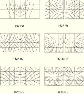
The first six nonzero frequencies are shown in Table 2.4.1–1, where they are compared with the calculated and experimentally measured values given by Petyt et al. (1977). There is fairly close agreement between all of the results, with the second-order model mostly providing higher frequencies (about 2% higher than those obtained with the first-order model). The pressure distributions predicted for these first six modes are shown in Figure 2.4.1–2.
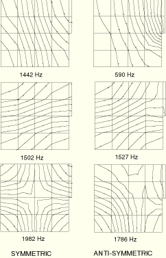
The half-model that takes advantage of symmetry provides identical results, as shown in Figure 2.4.1–3. Modes 2, 3, and 6 are obtained in the first step with the symmetry condition and modes 1, 4, and 5 are obtained in the second step with the antisymmetry condition.
AC2D4 elements.
AC2D8 elements.
The same problem as acousticmodes_ac2d4.inp with appropriate boundary conditions so that only half the cavity need be modeled.
Petyt, M., G. H. Koopman, and R. J. Pinnington, “Acoustic Modes of a Rectangular Cavity with a Rigid, Incomplete Partition,” Journal of Sound and Vibration, vol. 53, pp. 71–82, 1977.