Dynamic Queue Control Functions for ATM ABR Switch Schemes: Design and Analysis ¹ ² ³

Bobby Vandalore, Raj Jain, Rohit Goyal, Sonia Fahmy
The Ohio State University
Department of Computer and Information Science
Columbus, OH 43210-1277
Contact Phone: 614-292-3989, Fax: 614-292-2911
E-mail: {vandalor,jain, goyal, fahmy}@cse.wustl.edu

Abstract

The main goals of a switch scheme are high utilization, low queuing delay and fairness. To achieve high utilization the switch scheme can maintain non-zero (small) queues in steady state which can be used if the sources do not have data to send. Queue length (delay) can be controlled if part of the link capacity is used for draining queues in the event of queue build up. In most schemes a simple threshold function is used for queue control. Better control of the queue and hence delay can be achieved by using sophisticated queue control functions. It is very important to design and analyze such queue control functions. We study step, linear, hyperbolic and inverse hyperbolic queue control functions. Analytical explanation and simulation results consistent with analysis are presented. From the study, we conclude that inverse hyperbolic is the best control function and to reduce complexity the linear control function can be used since it performs satisfactorily in most cases.

Keywords:ATM Switch algorithms, ABR service, congestion control, traffic management, queue management.

Introduction

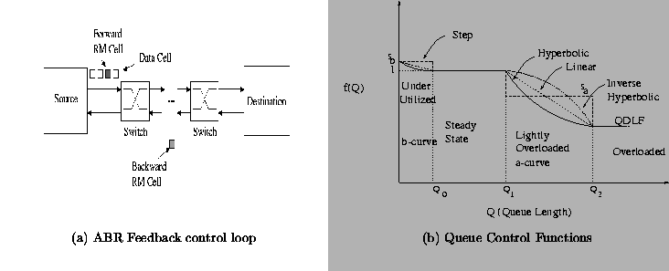
The ATM (asynchronous transfer mode) is the chosen technology for implementing B-ISDN (broad-band integrated services digital network). The ABR service in ATM can be used to transport data traffic with minimum rate guarantee. ABR uses closed loop feedback to control the source rates (see Figure 1 (a)). The source sends periodically (after every Nrm-1 data cells) an RM (resource management) cell to gather information from the network [ 1]. The RM cells are turned around at the destination. The switches along the path indicate the rate which they can currently support. When the source receives the backward RM cell, it adjusts its allowed cell rate based on the explicit rate indicated in the RM cell.

The goals of a rate allocation scheme are to maintain high utilization, small queuing delay, small cell loss, and fairness among competing sources. In order to support (low quality) video sources over ABR (Available Bit Rate) service, it is also desirable that in the steady state, the rates and queuing delay be constant. One way to achieve a high utilization and low queuing delay is to vary the target rate as a function of queue length. The function should be a decreasing function of queue length. The function should also be simpleso that it can be implemented in the hardware.

In this paper, we study several queue controlfunctions which satisfy the above needs. We present an analytical explanation for the performance of these functions. Then, we present simulation results which are consistent with the analysis. The various trade-offs between the queue control functions are studied using appropriate metrics. The ERICA+[ 2] switch scheme is used in the simulations.

Switch Scheme Model

There are many ABR switch schemes ([ 2, 3, 4, 5, 6]).

This section gives an overview of the switching scheme model on which this study is based.

An ABR switch scheme achieves the goals by giving explicit feedback to the sources to adjust their source rates. This type of switch is usually known as a Explicit Rate Feedbackswitch.
One way to achieve high utilization (100%) and control queuing delay by quick draining of queues is, to vary the target ABR rate dynamically. During the steady state, the target ABR rate is 100% while it is lower during the transient state. Higher overloads result in even lower target rates (thereby draining the queues faster). In other words:
Target rate = f(queue length) function (current rate, link rate, HPR)
HPR is the total rate of higher priority classes like VBR (variable bit rate) and CBR (constant bit rate). The ``f(queue length)'' has to be a decreasing function of the queue length. The switch scheme uses the above queue control function to adjust the allocated rate depending on the current switch queue size.
The switch measures the load, queue length and gives explicit feedback of target rate at fixed intervals. This interval is called the ``averaging interval''. The measurements are done using the FRMcells and the feedback is given using the BRMcells. We assume that only one feedback is given in each averaging interval to the sources. This avoids unnecessary conflicting feedbacks to the sources.

The ERICA+algorithm used in this study fits the above model.

Queue control functions

In this section the relationship between the queue length and queue control function is presented for the above switch model. Then various queue control functions to achieve the desired goals are presented.

The following terms are used in the discussion:

N: number of sources.
t_s: ``averaging interval'', the period at which feedback to the sources is calculated at the switch.
r_i(t): rate of source i.
er_i(t): explicit rate of source icalculated at the switch.
t_p: propagation time from the source to switch.
t_f: feedback delay is twice t_p.
R_l: Available ABR capacity. For simplicity we assume the higher priority traffic such as CBR and VBR are not present. Hence, R_lis same as the link rate.
Q(t): switch queue length (in cells)
R(t): aggregate input rateseen at switch.
C(t): (conversion function) number of cells transmitted in time tat link rate. if R_lis given in Mbps.

Note : X(t) denotes that Xis a function of time.

Queue Length Function

For the simplification of the analysis, we assume that the propagation delay t_pfrom source to switch switch is same for all sources. Due to propagation delay t_p, the rate seen at the switch at time tis the same as source rate at time t- t_p. The sources adjust their rates to the explicit rate indicated in the BRM cells. Due to propagation delay propagation delay t_pthe sources adjust their rate at time tto the explicit rate generated at time t-t_p. In one averaging interval Q(t) is drained by

cells. The queue builds up at input rate. Then, Q(t)can be expressed as follows :

Q(t) = Q(t-t_s) + (R(t) - R_l) C(t_s)

The switch scheme tries to adjust the input rate R(t) to match the output rate depending on current queue size, i.e., . We assume no higher priority traffic, so . Hence,

Q(t) = Q(t-t_s) + (f(Q(t-t_s)) - 1) R_lC(t_s)

and (f(Q(t-t_s)) - 1) R_lis the rate at which the queue changes in one averaging interval. The function f(Q) is the queue control function. The queue length increases if f(Q) > 1, remains constant if f(Q) = 1, and decreases if f(Q) < 1. Hence, by using an appropriate function f(Q), the queue length can be controlled.

Explicit Rate Feedback

The explicit rate is calculated as follows

The sources adjust their rates r_i(t) based on the explicit rate feedback from the switch. The feedback reaches the switch after time t_p. Hence, r_i(t) (source rate) can be expressed using the following equation ;

Since t_f= 2 t_p, we get

For simplicity we have assumed there is no HPR traffic (Note in the presence of bursty VBR sources there might not be any steady state of the system). So the above function becomes

For ERICA+scheme the above function is as follows

where Input Rateis the ABR input rate measured at the switch. The scheme tries to match the input rate to the link rate, by over allocating the rates if the queue is small. If the queue are large, it is drained quickly by using (1-f(Q)) part of the link capacity.

For other schemes the following modification can be done to incorporate queue control function with that scheme. Let er_A(t) be explicit rate calculated by an algorithm A. Then add the following as last step in the algorithm A:

where PCR is the peak cell rate. It can be shown that if the algorithm Aconverges to max-min rates, then the modified algorithm also converges to the max-min rate. Further, the queue control function f(Q) can be chosen so that the queue length (and hence delay) is constant in steady state.

Design of Queue Control Function

The design considerations for the queue control functions are as follows:

If queue length is very small it should be increased, so that the scheme can maintain some small queue which can used when the link is under utilized. This implies that f(Q) should be greater than one for small queue lengths.
In the steady state, we desire that the queue length be constant and the target rate to be the max-min fairness rate. The function Q(t) satisfies this goal if f(Q) = 1 in the steady state.
If the queue is large then part of the link capacity is used to drain the queue. Hence f(Q) should be less than one. It is desirable not to use all the capacity to drain the queue. Therefore, there is a minimum threshold, the queue drain limit factor (QDLF), for f(Q).
The f(Q) function has to be continuous. Discontinuities imply sudden changes which give rise to oscillations.

The queue control function with above properties will be of the form

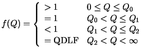
where

The following functions are possible candidates.

Step function
The step function has multiple thresholds (See figure 1 (b)). This is the simplest one to implement in hardware (lookup table).

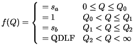
where s_a> 1 and are step parameters. In general it can have nsteps. In the above case n= 4.

Linear function
The function f(Q) has linear relationship with queue length. (See figure 1 (b))

where m_band m_aare slope of the linear portions. This function can be implemented in an efficient manner, using shift operations, if m_aand m_bare of the form 1/2^kand the queue length is counted in terms of Q₀.

Hyperbolic function
The function f(Q) is a hyperbolic function of the queue length. (See figure 1 (b))

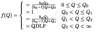
where h_aand h_bare the parameters which control the degree of curvature of the hyperbolic function. This function takes more time to calculate, since it has a division operation. For a high value of h_athe hyperbolic function becomes similar to the step function. For an h_avalue near 1, the hyperbolic function approaches the linear function.

Inverse Hyperbolic function
The fraction f(Q) is an inverse hyperbolic function of the queue length for overload conditions (see Figure 1 (b)). In the underload region, an hyperbolic function is used.

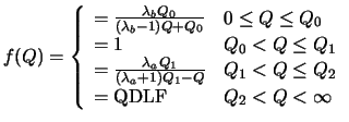
where and are the parameters which control the degree of curvature of the inverse hyperbolic and hyperbolic functions. This function is continuous and smooth at both Q₀and Q₁.

The curve used in the control function in underload region is called the ``a-curve'' and the one used in over loaded region is called the ``b-curve''. The parameters used in the a-curve are called a-parameters. are called the b-parameters. Note that, since all the functions are continuous, at Q₂we have the equation f(Q₂) = QDLF. So, Q₂can be expressed in terms of QDLFand a-parameterfor linear, hyperbolic and inverse hyperbolic functions.

**Figure 1:** Feedback Control and Queue Control Functions

Metrics

To compare the performance of the queue control function the following metrics are chosen.

Convergence Time:: The time the scheme takes to converge to steady state. To find the convergence time, the variance and standard deviation of desired variable are calculated between ( , ) for , where t_k( = 100 ms) is a small time interval). Initially the standard deviation is large due to oscillations. The convergence time is after which the variance is small. Also the graphs of (mean+standard deviation) value of the variable versus time are plotted. From the graph the convergence time can be calculated.
Standard Deviation:: The standard deviation of various quantities like ACRs, queue length and utilization is calculated. In order to separate the oscillations before steady state from affecting the measurement, the variance is measured both before and after steady state is achieved.

Visual inspection of the graphs also gives a good idea about the convergence time and the variations.

Analytical Explanation

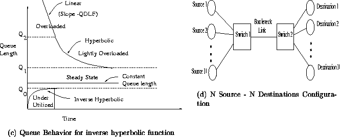
In this section we analyze the behavior of the proposed queue control functions. We assume a simple configuration in our analysis. Ninfinite ABR sources (always having data to send) are sending data to NABR destinations (See figure 2). The performance study under more stressful conditions is done by a simulation using the Generic Fairness configuration - 2 [ 7] in the section 7.

**Figure 2:**

The change in queue length in a averaging interval t_sis given by:

Initial behavior:In the beginning, the queue lengths grow depending on the initial ICR (initial cell rate). So the maximum queue depends on the ICR and round trip time and is independent of the queue control function used. The feedback information reaches the sources and the sources adjust their rates accordingly.
Under utilized:The switch initially estimates that the link is under utilized. The queue control function during under utilization is f(Q) > 1 for Q< Q₀. So, the switch gives feedback to the sources to increase their rates. Due to the increased rates the queue length at the switches increase. The rate of increase of the queue length is dictated by the b-curve of the queue control function.
Over loaded:Either due to the increase in the source rates or due to the high ICRs an overload condition occurs and queues at the switch grow. Initially the feedback information is not accurate; hence the queue might grow beyond the Q₂threshold. In such a heavy overloaded condition, the queues are quickly drained by using the (1-QDLF) fraction of the link capacity. In the meantime the feedback control loop is established, and the switch gives reliable feedback to the sources. For the lightly over loaded region, i.e., queue length in range of , the a-curve is the queue control function. The value of f(Q) is less than one in this region, which effectively decrease the queue length.
Steady state:The feedback information tries to match the input rate to output rate. As the input rate approaches output, rate the oscillations die down and the network reaches steady state. In the steady state, the rates and the queue lengths remain constant, since f(Q) = 1

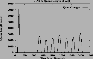
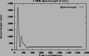
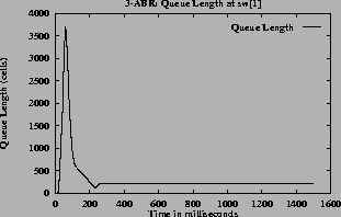
It is shown in [ 8] that additive increase and additive decrease leads to the steady state. For all four queue control functions f(Q) > 1 for and f(Q) < 1 for . The change in queue length depends on the value of f(Q) - 1. Hence, the change in the queue length is an additive increase for under utilized region and an additive decrease in the over loaded region. Therefore, the queue length converges to a value between Q₀and Q₁. An interesting point to note is that the amount of increase and the amount of decrease itself is dictated by the current queue length and its distance from the steady state queue length range. The behavior of the queue length for the inverse hyperbolic function is shown in figure 2 (a). The figure shows the queue length (y-axis) versus time (x-axis). The queue length decreases linearly in the range (highly overloaded) with slope QDLF. For queue length in the range (lightly overloaded, near the steady state) the slope is given by f(Q) - 1. Hence, the queue decreases hyperbolically (inverse of f(Q) function of a-curve) with respect to time. In the steady state, ( ) the queue length is constant. In under utilized range , the queue increases inverse hyperbolically since the slope is f(Q) - 1and f(Q) is hyperbolic.

Step Function

If Q(t-t_f) < Q₀then f(Q(t-t_f) = s_b> 1, so the queue grows till feedback information is passed to the sources asking them to decrease their rate. The queue grows for t_ftime and it can be expressed as follows:

If the condition Q₀< Q(t) < Q₁is satisfied and the input rate matches the output rate, then the steady state is achieved, and the queue remains at this constant length.

If Q₁< Q(t) < Q₂then the Q(t) starts decreasing with slope -(1-s_a). This decrease also takes place for t_ftime, if the queue ends up between Q₀and Q₁and if input rate is close to output rate then again the steady state is achieved.

Therefore, for the system to achieve the steady state, the value of queue length after one feedback interval should be within the range Q₀and Q₁. This requirement is satisfied if the condition holds. Since step function has discontinuities, it is very sensitive to queue length value near the thresholds and steady state might not be reached if the parameters are not set properly. If parameters are not set properly, then the queue grows from a value below Q₀for t_ftime, crosses Q₁, and decreases for t_ftime to a value less than Q₀. Then, this pattern repeats.

Linear Function

If Q(t-t_f) < Q₀, then f(Q(t)) > 1. Similar to the step function the queue keeps growing for t_ftime with a slope of

. But unlike the step function, the slope now depends on the value of queue length. After t_fseconds, if the queue Q(t) > Q₁, the queue length starts decreasing with a slope of

. The slope now depends on the value of the queue length so the there are no sudden changes in the slope. Therefore the oscillations are fewer when compared to the step function. If the system is near the steady state, then the oscillations decrease, the queue length reaches a value between Q₀and Q₁, and system reaches the steady state.

Hyperbolic Function

The analysis for this case is similar to above. If h_aand h_bparameter are close to one (typical values are h_a= 1.15, h_b= 1.05) the hyperbolic function has similar behavior as the linear function. If h_ais high then the hyperbolic function is close to the step function. Since the hyperbolic function has a larger curvature initially and then smoothes out,

value will be smaller than corresponding

value obtained using the linear function. Hence, the fluctuations in the rates are greater, but the queue draining is faster.

Inverse Hyperbolic Function

The behavior of the queue length versus time for the inverse hyperbolic function is shown in figure 2 (a). The behavior of this queue control function has been explained earlier in this section. Since the inverse hyperbolic function is continuous and smooth near Q₁, it gives rise to less oscillations compared to other cases.

Simulation: Configuration and Parameters

In this section the two configurations used in the simulations are explained. In all the simulation no higher priority (CBR and VBR) traffic is present.

Simple Configuration: N Source - N Destinations

In this configuration: (See figure 2)

N infinite sources send data to N destinations
The traffic is one way
The initial values of ICR are chosen randomly in the range (0,link rate)
All links are of length 1000 Km, which corresponds to a propagation delay of 5 ms.
All links have a bandwidth of 149.76 Mbps (after accounting for SONET overhead).
The sources start at random time between (0, t_RTT), where t_RTTis the round trip time. t_RTT= 30 ms for the above configuration.

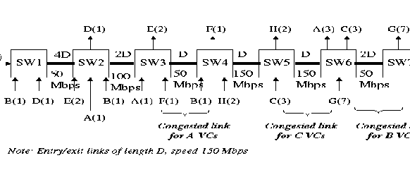
Generic Fairness Configuration - 2 (GFC-2)

This configuration (See figure 3) was used to test the performance of the queue control functions and the switch scheme under more stressful conditions. The value of link distance D was chosen to be 1000 Km. In this configuration the expected max-min fairness rate for the different VC's are: A VCs = 10 Mbps, B VCs = 5 Mbps, C VCs = 35 Mbs, D VC = 35 Mbps, E VCs = 35 Mbps, F VC = 10 Mbps, G VCs = 25 Mbps, H VCs = 52.5. This configuration is explained more in [ 7].

**Figure 3:** Generic Fairness Configuration - 2

Simulation: Results

In this section the simulation results using the above two configurations are given. The graphs of rates, queue length and utilization are given. The tables and the graphs are used to study the performance of different queue control functions. In the simulations for both configurations, QDLFwas chosen to be 0.5.

Simple Configuration: Results

The table 1shows the performance for different step values (parameters) of the step queue control functions as the queue threshold Q₁is varied. The mean bottleneck link queue length, its standard deviation before one second and after one second (last two columns) are shown in the table. Note that Q₂is fixed given the QDLFand other parameters of the linearand hyperbolicfunctions. Number of sources N= 3.

**Table 1:** Simple Configuration: Results
Queue	a	b	Q₁	Q₂	Convg	Mean	Std Dev	Std Dev
Control	param	param			time(secs)	Q(cells)	(bef 1 sec)	(after 1 sec)
Step	0.75	1.01	4 Q₀	26 Q₀	-	252.93	552.21017	501.60
	0.90	1.01	4 Q₀	26 Q₀	-	98.04	651.82	241.43
	0.90	1.05	4 Q₀	26 Q₀	-	663.63	1226.70	840.36
	0.95	1.01	4 Q₀	26 Q₀	-	251.51	816.62	393.26
	0.95	1.05	4 Q₀	26 Q₀	-	124.11	805.32	240.04
	0.95	1.01	2 Q₀	26 Q₀	-	896.90	1386.87	1036.66
	0.95	1.01	8 Q₀	26 Q₀	-	483.20	1001.54	644.73
Linear	1/16	1/16	2 Q₀	26 Q₀	0.20	311.85	335.61	0.69
	1/16	1/16	4 Q₀	26 Q₀	0.32	403.52	457.90	0.69
	1/16	1/16	8 Q₀	26 Q₀	0.61	402.85	622.02	0.69
Hyperbolic	1.15	1.05	2 Q₀	26 Q₀	-	509.94	423.89	205.65
	1.15	1.05	4 Q₀	26 Q₀	0.32	214.19	500.14	0.86
	1.15	1.05	8 Q₀	26 Q₀	0.82	220.96	862.25	0.63
Inverse	36	1.05	2 Q₀	26 Q₀	0.22	313.17	525.51	0.69
Hyperbolic	16.5	1.05	4 Q₀	26 Q₀	0.25	209.50	580.15	0.50
	6.75	1.05	8 Q₀	26 Q₀	1.12	202.27	704.02	16.98

The following things can be observed from the Table 1.

The step function never converges entirely. The values are fluctuating near the target values, so the standard deviation after one second is lower than the standard deviation in the first second.
The linear and hyperbolic and inverse hyperbolic functions reach steady state after one second since the standard deviation after one second is very small.
As Q₁increases, the convergence time increases for the linear, hyperbolic and inverse hyperbolic functions
For Q₁= 2 Q₀, the linear function converged. The value of f(Q) for hyperbolic function value is less compared to that of linear function, so the queue is drained faster and Qbecomes less than Q₀. Therefore for the hyperbolic function the queue length and rate values are oscillating near the target value. This is mainly because the hyperbolic function is not smooth (not differentiable) near Q₁. The inverse hyperbolic is smooth at Q₁so the queue lengths do converge in this case.
For Q₁= 8 Q₀, the convergence time for hyperbolic function and inverse hyperbolic is more than linear. This happens since the both hyperbolic and inverse hyperbolic function vary slowly near the steady state. The queue length variance is more for the inverse hyperbolic function.

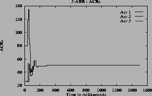
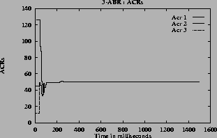
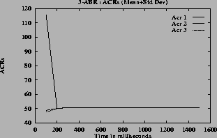
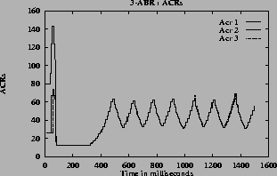
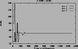
The graphs 4 (a), 4 (e), 5 (a), 5 (e) show the ACR rate of the three sources.

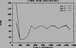
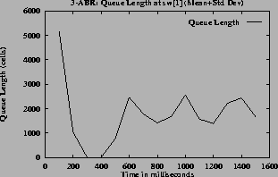
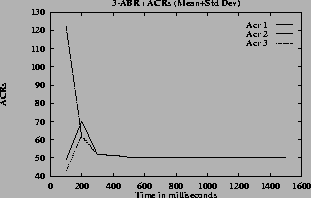
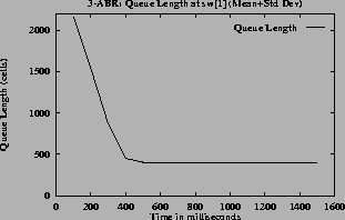
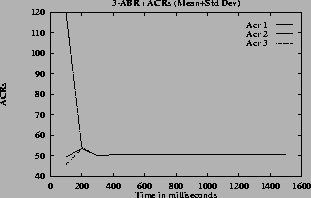
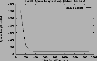
The mean and standard deviation of the rates and the queue lengths are calculated for every 100 milliseconds. These are shown in figures 4 (b), 4 (f), 5 (b) and 5 (f) for ACR rates and in figures 4 (d), 4 (h), 5 (h) for the queue lengths. From these graphs the converging time can be estimated. In steady state the oscillations are small, the standard deviation is small compared to mean. So the quantity (mean + standard deviation) has a value close to the mean in the steady state.

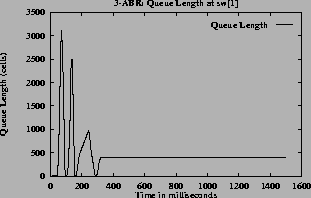
For the step function, there is oscillation in all the quantities (rates, queue and utilization). For linear and hyperbolic functions, the oscillations die down and the system reaches steady state. In the steady state, the rate and queue length are constant and utilization is 100%. Hence the linear, hyperbolicand inverse hyperbolicqueue control functions fulfill the desired goal. This is consistent with the analytical explanation given in the previous section.

In all the cases when the queue length and the rates converge, the queue length is non-zero hence, the utilization at the steady state is 100%.

GFC-2 Configuration: Results

The following parameters were used in the simulations for this configuration.

Thresholds: Q₀= 176, , , QDLF= 0.5
Step: s_a= 0.95, s_b= 1.01
Linear: m_a= 1/16, m_b= 1/16
Hyperbolic: h_a= 1.15, m _b= 1.05
Inverse Hyperbolic: ,

The table 2shows the performance for three queue control functions. The table shows the H(1) VC's mean rate, switch queue length for SW5 and its convergence time, standard deviation before one second and after one second. The queue length variation is present in all three cases. The rate variation is much less in the linearand hyperbolicfunctions compared to the stepfunction. This is also evident from the graphs which are explained in the next section.

**Table 2:** GFC-2 Configuration: Results
Queue	Quantity	Convergence	Mean	Std Dev	Std Dev
Control		Time (secs)		(before 1 sec)	(after 1 sec)
Step	H(1) ACR	-	72.81	18.4	4.46
	SW5 Queue	-	284.28	878.63	281.85
Linear	H(1) ACR	1.25	52.46	14.38	1.08
	SW5 Queue	1.3	455.46	1043.71	220.42
Hyperbolic	H(1) ACR	1.45	52.77	13.57	0.58
	SW5 Queue	1.3	361.32	968.27	201.86
Inverse Hyperbolic	H(1) ACR	1.51	52.38	14.04	0.92
	SW5 Queue	2.0	1443.72	3829.17	999.62

GFC-2 Configuration: Graphs

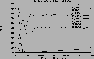
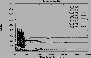
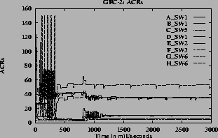
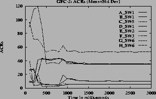
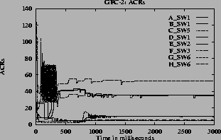
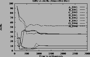
The graphs in Figure 6and 7were obtained by simulating the GFC-2 configuration using the step, linearand hyperbolicand inverse hyperbolicqueue control functions. Graphs 6 (a), 6 (e), 7 (a) and 7 (e) show the ACR rate for one VC of each of A through H type VCs versus time when different queue control functions are used. From these graphs it can be seen that the expected rates are obtained when linear, hyperbolic and inverse hyperbolic functions are used for queue control.

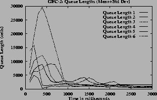
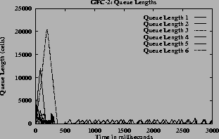
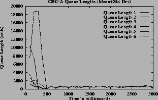
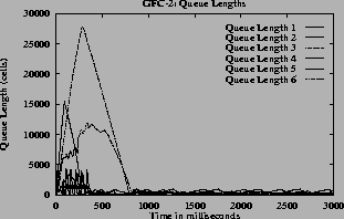
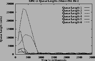
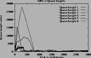
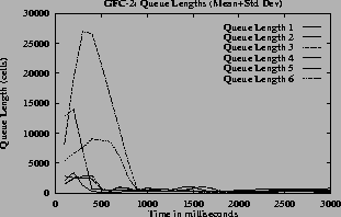
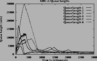
The (c) and (g) graphs have the queue length for all the switches. The maximum queue is due to the initial overload, before the first round trip time. Once the feedback control loop is established the f(Q)value is QDLFand queues are drained quickly.

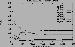
When step function (Figure 6 (b)) is used the oscillations are more compared to the oscillations when other functions are used. The graphs 6 (b), 6 (f), 7 (b), 7 (f) plot mean plus standard deviation for VC (ACR) rates. The figures 6 (d), 6 (h), 7 (d), 7 (h) plot corresponding (mean+standard deviation) graphs for the queue lengths.

Note that in the graphs when the step function is used, some of the VCs do not get their max-min fair share rates and the VCs near the fair share have considerable oscillations. The step function is very sensitive to queue length variation near the thresholds. Since the configuration is complex, with large number of VCs passing through each of the switches, the queue length and hence the rates vary. For the graphs 6 (e), 7 (a) and 7the oscillations are only present before steady state. The oscillations die down and the rates become steady since the function f(Q) changes smoothly. The maximum queue length is same for all queue control functions since this depends only on the ICR. When the inverse hyperbolic function is used the queues are larger since in this case the steady state queue length is near Q₁.

Figure 4: Simple Configuration: Rate, Queue and Utilization graphs: Step and Linear queue control function

[] []
[] []
[] []
[] []

Figure 5: Simple Configuration: Rate, Queue and Utilization graphs: Hyperbolic and Inverse Hyperbolic queue control function

[] []
[] []
[] []
[] []

Figure 6: GFC-2 Configuration: Rate, Queue and Utilization graphs: Step and Linear queue control function

[] $\includegraphics[height=2.8in,angle=-90]{/home/cong/tests/param/1997/ERICA_SIMS/gfc2.snapfile,step,14403,3000000,0.9,1.01,0.95,26,4,1,1,DIR/r.ps}$ []
[] []
[] []
[] []

Figure 7: GFC-2 Configuration:: Rate, Queue and Utilization graphs: Hyperbolic and Inverse Hyperbolic queue control function

[] []
[] []
[] []
[] []

Summary of Results

The simulation results obtained by using different queue control functions in the simple and the GFC-2 configurations are consistent with the analytical explanation. The step function is sensitive to queue thresholds ( Q₀,Q₁,Q₂) used. The other functions are not sensitive to these queue thresholds. Small steady state queuing delay can be achieved by choosing nearby values for Q₀and Q₁.

Conclusion

In this paper we have considered the problem of designing a simple and robust queue control function for switch schemes. A switch scheme tries to maximize utilization, minimize queuing delay and give max-min fair rates to the sources. It is also desirable to have less oscillations in rates and queue length to support (low quality) video over ABR service. We assume a switch scheme model which dynamically adjusts the rate of the sources to match the output rate and drain large queues. The design considerations were discussed with analytical explanations. Four different queue control functions were analyzed. The choice of parameters for the queue control functions was both explored analytically and by simulation. The simulation showed that even in complex configuration (like GFC-2) the system behavior was consistent with of the analytical explanation. When the step function is used, the systems oscillates and does not converge in most cases. From both the analytical and the simulation results, it can be concluded that the inverse hyperbolic is the best queue control function, followed by the hyperbolic and the linear queue control functions. For simpler implementation complexity, the linear function is recommended.

Bibliography

1: The ATM Forum.
The ATM forum traffic management specification version 4.0.
ftp://ftp.atmforum.com/pub/approved-specs/af-tm-0056.000.ps, April 1996.
2: S. Kalyanaraman, R. Jain, S. Fahmy, R. Goyal, and B. Vandalore ⁴.
The ERICA switch algorithm for ABR traffic management in ATM networks.
Submitted to IEEE/ACM Transactions on Networking, Nov. 1997.
3: L. Roberts.
Enhanced PCRA (Proportional Rate Control Algorithm).
ATM Forum/AF-TM 94-0735R1, 1994.
4: Ambalavanar Arulambalam, Xiaoqiang Chen, and Nirwan Ansari.
Allocating fair rates for available bit rate service in ATM networks.
IEEE Communications Magazine, 34(11):92-100, November 1996.
5: Y. Afek, Y. Mansour and Z. Ostfeld.
Phantom: A simple and effective flow control scheme.
In Proc. of the ACM SIGCOMM, August 1996.
6: A. W. Barnhart.
Example Switch Algorithm for TM Spec.
ATM Forum 95-0195, Feburary 1995.
7: Robert J. Simcoe.
Test configurations for fairness and other tests.
ATM Forum/94-0557, July 1994.
8: D. Chiu and R. Jain.
Analysis of the increase/decrease algorithms for congestion avoidance in computer networks.
Computer Networks and ISDN, 17(1), June 1989.

Footnotes

... Analysis ¹: Based on ``Design and Analysis of Queue Control Functions for Explicit Rate Switch Schemes'', Bobby Vandalore, Raj Jain, Rohit Goyal, Sonia Fahmy, Proceedings of International Conference on Computer and Communications Networks (IC3N), October 12-15, 1998, Lafayette, Lousiana, pp. 780-786 ©1998 IEEE.
...1 ²: Submitted to Computer Networks and ISDN Systems, November 1998.
...2 ³: This research was sponsored in part by Rome Laboratory/C3BC Contract #F30602-96-C-0156.
... Vandalore ⁴: All our papers and ATM Forum contributions are available through http://www.cse.wustl.edu/~jain/index.html

Bobby Vandalore
1999-02-18