| Zhuangyu Han (A paper written under the guidance of Prof. Raj Jain) |
Download |
Keywords: quantum communication, qubit, quantum entropy, quantum teleportation (QT), superdense coding (SDC), quantum key distribution (QKD), BB84, satellite-based quantum channel
From the beginning of the 20th century, quantum physics is always an attractive discipline. The group of
experiments about the unpredictable position of a particle and superposition of distribution density makes most of
the people confused and surprised when they see such a phenomenon for the first time. An electron knows whether
there is a wall before it hit the wall! Also, we can even not regard an electron as a particle before we
see it detected because interacting with any piece of space where the wave function has non-zero value
will change the state of an electron [Carnal91]. Quantum mechanics describes the states of a quantum
system by vectors in Hilbert space, which will be defined below. All the observables can be represented
by matrices or operators, which could be applied to a state vector or a density operator of a mixed
state.
Quantum communication is a new field, in terms of communication, where people send or receive messages by
transmitting quantum states of a specific quantum system, for example, a photon. Photons can be sent through free
space or optical fibers. The quantum states are the physical characteristics of the photons, such as polarization. A
45-degree linearly polarized beam could penetrate a vertical polarizer with 50 percent energy loss. However, if
people send photons in the same polarization state one by one to the polarizer, either zero or one photon will be
observed with probability both 50 percent. Such a phenomenon can only interpreted by quantum mechanics with
probability. The difference between quantum communication and classical communication is that the
characteristics of quantum systems allow people to detect any traditional eavesdropping theoretically
[Wilde13]. As eavesdropping on a mixed state of a quantum system will certainly destroy the state, we
could design protocols where we have ways to detect adversaries by checking whether a mixed state is
changed.
In Section 2, the fundamental knowledge of mathematics and information theory is necessary for quantum communication. From the quantum information theory, we could find some extraordinary features of quantum systems. Then quantum teleportation (QT), which is the transmission of a pure state with the help of classical channels [Pathak13], and superdense coding (SDC), which allows us to encode m bits of classical information with n qubit, where n < m [Pathak13], will be introduced. In Section 5, the basic concepts of QKD will be presented. QKD is a hot topic these years, but the first protocol of QKD can date back to 1984 [Bennett84]. QKD allows us to share a key used to encrypt information which can be transmitted in classical channels. The point is that once there is an adversary who eavesdropped on the key, it will be detected definitely (with probability arbitrarily close to 1). In the last section, some recent advances of quantum communication will be presented including satellite-based QKD [Liao17] and free-space quantum channel in daylight [Liao17a].
In this section, some basic mathematics tools for dealing with quantum systems will be introduced. The Hilbert space where all the possible quantum states are vectors on it is the most important concept. Then, all the physics observables such as spin, position, and polarization direction are Hermitian matrices. Next, a density operator for a mixed state contains all the information of such a state. It is easy to calculate the expectation of an observable of a mixed state by its density operator. Then the most popular implementation of a qubit will be given.
Hilbert space is very similar to Euclidean space, but the elements of Hilbert space could be complex, and there is an
inner product defined on it.
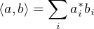
Definition: An element of a d-dimensional Hilbert space ℍ is a d-tuple

The inner project defined in such a space is that
![⌊ ⌋
|b1|
⟨a,b⟩ = [a* a* ... a*]||b2||
1 2 d ⌈... ⌉
bd](fig2.png)
Obviously, ⟨a,a⟩∈ ℝ and is non-negative for any vector a in H.
Definition: The valid quantum states is the following set of vectors
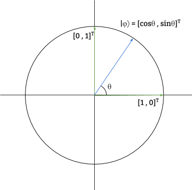
For example, almost the simplest quantum system is called a quantum bit or a qubit, whose state can be
represented by a vector in 2-dimensional Hilbert space.
E.g. [10]T is a state vector for a single qubit.
A state vector of a single qubit has a general form
![[ ]
α 2 2
β α,β ∈ ℂ,|α| + |β| = 1](fig4.png)
A qubit is an analog to a classical bit, such as a bit in our PCs’ memory. The states of a qubit corresponding to the
two states of a classical bit are [10]T,[01]T, which represents classical 0 and classical 1.
However, a qubit could be in a state as a superposition of classical states, for example  (
(![[ ]
1
0](fig6.png) +
+ ![[ ]
0
1](fig7.png) ) =
) = ![[ 1-]
√12
√2-](fig8.png) and
and

![[1]
0](fig10.png) +
+ 
![[0]
1](fig12.png) =
= ![[ 12√-]
-3-
2](fig13.png) .
.
In quantum mechanics, we usually use |ϕ⟩ to represent a state vector and ⟨ϕ| to represent the conjugate transpose of the same state vector. They are called the Dirac notation. And we write the inner product of two state vector |ϕ⟩ and |ψ⟩ as ⟨ϕ|ψ⟩ The joint state of two systems could be written as |ϕ,ψ⟩ = |ϕ⟩⊗|ψ⟩ Where ⊗ is the tensor product. In matrix form,
![⌊a a ⌋
[a ] [a ] [a ] [a ] |a1b2|
|ϕ ⟩ = b1 |ψ⟩ = 2b ⇒ |ϕ,ψ⟩ = |ϕ⟩⊗ |ψ⟩ = b1 ⊗ 2b = |⌈b1a2|⌉
1 2 1 2 b1b2
1 2](fig14.png)
When measuring such states not corresponding to classical 0 (![[1]
0](fig15.png) ) and 1 (
) and 1 (![[0]
1](fig16.png) ) are measured, the possibility of
getting 0 and getting 1 are both non-zero, which means sometimes 0 could be observed, and sometimes 1 could be
observed from the devices. For the general form of a state of a qubit,
) are measured, the possibility of
getting 0 and getting 1 are both non-zero, which means sometimes 0 could be observed, and sometimes 1 could be
observed from the devices. For the general form of a state of a qubit, ![[ ]
α
β](fig17.png) , the probability of getting 0 is |α|2, and
the probability getting 1 is |β|2.
, the probability of getting 0 is |α|2, and
the probability getting 1 is |β|2.
When we are talking about measurement, there is always a group of orthonormal basis

This set of basis depends on the observable being measured. When we measure the position of a
particle, we will have a set of basis that is different to the basis used to measure the momentum. The
measurement will always make a quantum system be into a basis state. Besides, a state that is not
a basis state, but the weighted sum of multiple bases states is measured, the superposition will be
destroyed.
For example, if state [
 ]T is measured with computational bases [10]T,[01]T. [10]T or [01]T with probability
both
]T is measured with computational bases [10]T,[01]T. [10]T or [01]T with probability
both  will be observed. This indicated that the measurement makes the state of a quantum system collapse into
one of the bases related to the measurement, and we could observe that the basis it collapsed into after
measurement. Quantum measurement will change the state if a system but classical measurement will not. From
next part, it shows that the measurement result is the eigenvalue corresponding to the basis state, of a
matrix.
will be observed. This indicated that the measurement makes the state of a quantum system collapse into
one of the bases related to the measurement, and we could observe that the basis it collapsed into after
measurement. Quantum measurement will change the state if a system but classical measurement will not. From
next part, it shows that the measurement result is the eigenvalue corresponding to the basis state, of a
matrix.
Observables are physical quantities that can be measured, such as position, momentum, and spin of a particle. The
value of a qubit is also an observable because we could measure to see that it is classical 0 or classical 1. In quantum
mechanics, an observable is always related to a hermitian operator, which actually is a hermitian matrix when we
are using linear algebra.
Definition: A is a hermitian matrix, if

If A is a hermitian matrix and λ is an eigenvalue of A with corresponding unit length eigenvector v, we have

The measured value of a qubit is again a good example to an observable. The two bases of the measurement of a qubit here are the computational basis
![[ ] [ ]
|0⟩ = 1 ,|1⟩ = 0
0 1](fig24.png)
![[ ]
C = 1 0
0 - 1](fig25.png)


Operators are important tools for the analysis of a state.
If we know that a quantum system is in a certain state, this system is called in a pure state. For example, a qubit
could be in |+⟩ = [
 ] or |-⟩ = [
 -
- ]. Both |+⟩ and |-⟩ are superpositions of bases states, but the state is
determined to us, so they are called pure states.
]. Both |+⟩ and |-⟩ are superpositions of bases states, but the state is
determined to us, so they are called pure states.
If we cannot determine the state of a system, we say that this system is in a mixed state. For example, if we
can only know that a qubit is in |+⟩ with probability  and in|1⟩ with probability
  as well, we say
that this qubit is in a mixed state. Obviously, the set of pure states is a subset of the set of mixed
states.
as well, we say
that this qubit is in a mixed state. Obviously, the set of pure states is a subset of the set of mixed
states.
To conveniently represent a mixed state, we usually use a density operator. If we know the possible pure state |ϕi⟩i = 1,2,... and corresponding probability pi, we have the density operator for this mixed state
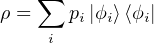
The expectation of an observable A of a mixed state ρ is Tr(Aρ), where Tr(M) is the trace of M
[Cariolaro15].
The density operators are useful when we are talking about the entropy of a quantum system.
There are several ways to implement a qubit quantum system. The most popular approach is to use the polarization
states of photons. We could code |0⟩ into horizontal polarization and code |1⟩ into vertical polarization. A photon
can be in a superposition state of horizontal and vertical polarization. Here the 45-degree tilted linear polarized
photons are in the |+⟩ or |-⟩ state. We could also use the spin of an electron or a nuclear to represent a qubit. The
spin of a nuclear can be measured by the magnetic field. The nuclears with different spin will hit distinct spots after going
through a magnetic field.
When it comes to the transmission of a qubit, there are many approaches, as well. Here only photon-based implementation will be discussed. We could use the optical fiber [Lucamarini18] or free-space [Liao17a] as the medium of the quantum transmission. The optical fiber is commonly used for the internet. Lasers are handy sources of photons because the spectrums of lasers are super narrow (~ 0.02nm) [King77]. We can use optical devices such as polarizers, beam splitters, and photon detectors, to modulate and detected photons.
Generally speaking, we use unit vectors in Hilbert space ℍ to represent quantum states. The observables are hermitian matrices, which could be applied to a state vector to get the possible measured values or the expectation value corresponding to the states. A density matrix/operator is used to represent a mixed state. When we are implementing a qubit, we could usually use the polarized photons and transmit them in optical fibers or free space. In the next section, the amount of information contained in a qubit will be elaborated. Actually, it depends on the state of the qubits.
When people are talking about classical communication, the Shannon information theory plays an indispensable role in calculating the channel capacities the minimum number of bits for transmitting a message. In quantum communications, we use quantum entropy to calculate the amount of information contained in a qubit. There are also some interesting features of quantum information. A classical system does not have the counterpart of the features.
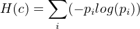
Shannon entropy [Shannon48] is a critical concept in classical communications. It is used to measure the amount of
information contained in the uncertainty of a symbol, a word, or a sequence.
Definition: If there is an alphabet Σ and for each element ai in this alphabet there is a corresponding probability pi to it, the classical entropy of a symbol c from this alphabet is
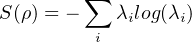
The quantum entropy, or Von Neumann entropy [Cariolaro15], is very similar to Shannon entropy. If, for a quantum
system, we do not exactly know the state of it but a distribution of all the possible states, we could
have its density matrix. The Von Neumann entropy is defined on the density matrix of a system.
Definition: If there is a quantum system whose density matrix is ρ, the Von Neumann entropy of this system is
![S(ρ) = - Tr[ρlog(ρ)]](fig38.png)
For example, [Cariolaro15], let us consider a qubit with probability  in the state |0⟩ and
  in the state |+⟩. The
density matrix of this mixed state is
in the state |+⟩. The
density matrix of this mixed state is
![[ ] [ ] [√- ]
1 1 1 1 0 -1-- 1 1 -1-- 2 + 1 1
ρ = 2 |0⟩⟨0|+ 2 |+ ⟩⟨+ | = 2 0 0 + 2√2- 1 1 = 2√2 1 1](fig42.png)

 , its entropy will be 1 bit. But for a quantum system, it is not necessarily 1
qubit.
, its entropy will be 1 bit. But for a quantum system, it is not necessarily 1
qubit.
Definition: Conditional entropy

This formula tells us that, in a joint system AB, if we have already known the state of system B, the total
information from this system will decrease and the remaining part is H(A|B). The more correlated A and B are, the
less information there is after knowing B. People will have a good guess of symbol A after people know symbol B is
these two symbols are strongly correlated.
In a classical joint system, a part of the system will never tell us the amount of information more than the information in the entire joint system, which could be expressed a non-negative conditional entropy
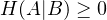
However, in a quantum system, the conditional quantum entropy could be negative, which implies that knowing a
part of a system could make a system more uncertain [Wilde13].
The definition of quantum joint entropy, quantum marginal entropy and quantum conditional entropy are Joint quantum entropy:
![S(AB) = - T r[ρABlog(ρAB)]](fig47.png)
![S (A ) = - Tr[ρAlog(ρA)] S (B ) = - Tr[ρBlog(ρB)]](fig48.png)

Definition: Bell state is
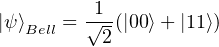
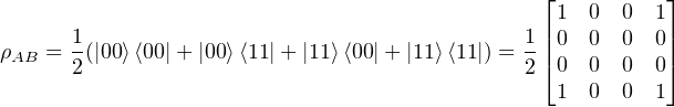
Then we know that the ρB =  I and it is easy to know that the Von Neumann entropy of qubit B is 1 qubit.
According to the formula S(A|B) = S(AB) - S(B), we have S(A|B) = -1.
I and it is easy to know that the Von Neumann entropy of qubit B is 1 qubit.
According to the formula S(A|B) = S(AB) - S(B), we have S(A|B) = -1.
The negative conditional quantum entropy is anti-intuitive, and the Nocloning theorem even tells us that a qubit
cannot be copied.
In quantum information theory, we have the Nocloning theorem, saying that we cannot copy a quantum state of a
system to another system without destroying the original version.
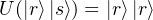
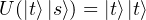
Theorem [Wilde13]: In a Hilbert space ℍ, there is not a unitary transformation U : ℍ ⊗ ℍ → ℍ ⊗ ℍ such that there exists a state |s⟩∈ ℍ satisfying

Proof: Assume that there is such a unitary matrix U realizing

This theorem tells us that an eavesdropper cannot copy a state and forward it without destroying the original version. In some aspects, this theorem reveals that quantum communication cannot be eavesdropped on in any traditional way.
In this section, some basic knowledge about quantum information theory is mentioned. The Shannon entropy measures the uncertainty of a classical symbol, and the Von Neumann entropy measures the information contained in a mixed state of a quantum system. We saw that a qubit having 2 equally possible states could contain less than 1 qubit of quantum information. Next, the conditional quantum entropy could be negative, which is a typical quantum characteristic and there is no classical counterpart. Finally, the state of a quantum system cannot be copied without destroying the original version. This quantum information feature guarantees the security of the quantum communication systems in some aspects. The extraordinary features of a quantum system enable us to realize many amazing applications such as QT, SDC, and QKD.
QT [Bennett93] and SDC [Bennett92] are two well-known applications of quantum mechanics. QT allows two people to transmit an unknown state of a qubit with the help of classical channels, but the sender (Alice) and the receiver (Bob) must initially share an entangled pair of qubits. SDC enables us to encode 2 bits of classical information with 1 qubit, but priorly it also needs entangled pairs. In the beginning, quantum gates and the concept of entanglement will be introduced which are indispensable for the following applications.
Quantum gates are just matrices like the operators introduced in Section 1. A quantum gate must be a unitary
matrix mapping one unit vector into another unit vector. When we apply a quantum gate to a qubit, the state of
the involved qubits will change. Below are several common quantum gates used in quantum communication and
quantum computing [Kaye07].
Identity gate:
![[ ]
I = 1 0
0 1](fig57.png)
Pauli X, Y, Z gates:
![[ ] [ ] [ ]
X = 0 1 Y = 0 - i Z = 1 0
1 0 i 0 0 - 1](fig58.png)
Hadamard gate:
![1--[1 1 ]
H = √2 1 - 1](fig59.png)
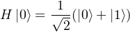
Example: If we apply a Hadamard gate onto a qubit in state |0⟩, we have
![[ ] [ ] [ ]
H |0⟩ = √1- 1 1 1 = √1- 1 = √1-(|0⟩+ |1⟩)
2 1 - 1 0 2 1 2](fig61.png)
![⌊ ⌋
[ ] [ ] 1
|0⟩⊗ |0⟩ = 1 ⊗ 1 = ||0|| = |00⟩
0 0 ⌈0⌉
0](fig62.png)
If we apply Hadamard gate to q1, we have
Now the joint state is
![⌊ ⌋
[ ] [ ] [ ] 1
-1- 1 0 1 1--||0||
√2-( 0 + 1 )⊗ 0 = √2 ⌈1⌉
0](fig64.png)
Then, If we apply CNOT gate onto q1 and q2 at the same time, we have

Next, we will use a diagram to show how does QT work.
QT allows us to transmit an unknown state of a qubit without really sending qubits in quantum channels. However,
Alice and Bob must previously share a pair of entangled qubits. I will give an example here to interpret the entire
transmission process [Wilde13].
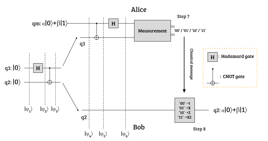
Figure 2 shows the quantum circuit used for teleportation. I will show the effect of applying quantum gates onto
the qubit step by step. The joint states of all the qubits will be shown after each step, like |ϕ1⟩, |ϕ2⟩
,...
(1) Here we have two independent qubits both in |0⟩ state.
(2) After the Hadamard gate is applied to q1, the joint state of q1 and a2 becomes

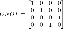
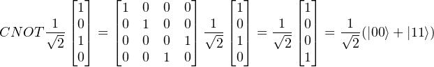
(3) Then we apply a CNOT gate to the two qubits.
![|ϕ3⟩ = CN OT |ϕ2⟩ = CN OT √1-[1010]T = √1-[1001]T
2 2](fig69.png)
which is just the Bell state.
(4) Then we send q1 to Alice and q2 to Bob with the joint state not changed. We introduce qm, the qubit we want to transmit whose state. As we do not know the state of qm, we assume that its state could be written as α|0⟩ + β |1⟩, where |α|2 + |β|2 = 1. The joint state of these three qubits is

(5) Then we apply the CNOT gate to qm and q1, we have

(6) Next, we apply a Hadamard gate to qm, we have
![1
|ϕ6⟩ = 2[α(|0⟩+ |1⟩) |00⟩+ α(|0⟩ + |1⟩)|11⟩+ β(|0⟩- |1⟩)|10⟩ + β(|0⟩- |1⟩)|01⟩]](fig72.png)
![1
= 2 [|00⟩(α |0⟩ +β |1⟩)+ |01⟩(α |1⟩+ β|0⟩)+ |10⟩(α|0⟩- β|1⟩) +|11⟩(α|1⟩- β|0⟩)]](fig73.png)
(7) If Alice measures qm and q1, she will have 4 possible outcomes 00, 01, 10, or 11. I call the result of Alice’s
measurement K.
(8) Alice tells Bob the K she got through a classical channel, for example an email. Bob applies a corresponding quantum gate to q2. Table 1 gives the state of q2 after step 7 and the corresponding gates.
Table. 1: The states after step 7 and the corresponding gates [Wilde13]
| K | State of q2 after step 7 | The gate applied to q2 by Bob | The final state of q2 |
| 00 | α|0⟩ + β |1⟩ | I | α|0⟩ + β |1⟩ |
| 01 | α|1⟩ + β |0⟩ | X | α|0⟩ + β |1⟩ |
| 10 | α|0⟩- β |1⟩ | Z | α|0⟩ + β |1⟩ |
| 11 | α|1⟩- β |0⟩ | ZX | α|0⟩ + β |1⟩ |
Now we find out that the state of q2 has become the same as the original state of qm. Certainly, the state of qm has changed because of the Nocloning theorem. This is what we called QT. Below SDC could realize information compression impossible in a classical communication system.
In this example of SDC, I will show that Alice could send Bob two classical bits with sending only one qubit. They
must previously share a pair of entangled qubits [Wilde13].
Firstly, we prepare two qubits q1 and q2, which are jointly in Bell state:  (|00⟩ + |11⟩), and send q1 to Alice, q2 to
Bob.
(|00⟩ + |11⟩), and send q1 to Alice, q2 to
Bob.
The two classical bits Alice want to send will be one of the following 4 values: ‘00’, ‘01’, ‘10’, ‘11’. For each
value Alice wants to send, there is a corresponding single-qubit unitary matrix that can be applied to
q1.
Then Alice applies the gate to q1, so we have the corresponding joint state of q1 and q2. For example, if Alice wants
to send ‘10’, she will use the gate iY.
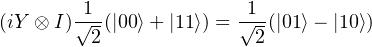
Table 2 shows all the joint state after applying the corresponding gate.
Table. 2: The gates applied to q1 and the corresponding final joint state [Wilde13]
| Value | Gate | The final joint state |
| 00 | I |  (|00⟩ + |11⟩) (|00⟩ + |11⟩) |
| 01 | X |  (|10⟩ + |01⟩) (|10⟩ + |01⟩) |
| 10 | iY |  (|01⟩-|10⟩) (|01⟩-|10⟩) |
| 11 | Z |  (|00⟩-|11⟩) (|00⟩-|11⟩) |
It is easy to check that the four possible final joint states, in the right column, of q1 and q2, are orthogonal to each
other, which compose a group of bases of the Hilbert space for 2 qubits. Now Alice will send q1 to Bob. Then Bob has
both q1 and q2.
Bob uses this group of bases to measure the q1-q2 system, and he will get one from the 4 bases with possibility one,
which is just like measuring a photon, either horizontally polarized or vertically polarized, by using a polarizer in
the horizontal direction.
As the result can be completely determined, Bob will know the value of two classical bits that Alice wants to send. In this process, Alice only sent one qubit to Bob after she determines her message, so this is called SDC. In total, Alice sends Bob 2 qubits, but the information could be coded into the first bit even after the first bit has been sent to Bob, which is amazing. This communication method could only be realized with quantum system.
In this section, two typical applications of quantum communications are described, QT and SDC. The former could send an unknown state from Alice to Bob with an existing pair of entangled qubits. The latter could encode two classical bits into one qubit with an existing pair of entangled qubits. In the next section, there is an overview of the most popular application of quantum cryptography, which is called quantum key distribution.
QKD allows us to share a common key for encrypting classical information, without being eavesdropped by the adversary in any traditional way. Eavesdropping the qubits in the quantum channel while distributing a key could be detected with probability arbitrarily close to 1. In some countries, banks have already deployed QKD systems for encrypting important messages transmitted between two cities [Zhang18]. Furthermore, recently there are lots of researches on QKD. A team has realized satellite-based QKD over thousands of miles [Liao17]. Others realized QKD in the noise background of sunlight [Liao17a].
BB84 protocol is a well-known protocol for QKD developed by Charles Bennett and Gilles Brassard in 1984
[Bennett84]. The below figure shows the diagram of a BB84 QKD system.
The example [Bennett84] of sending and receiving qubits are elaborated in the table below.
Table. 3: A BB84 example [Bennett84]
| Index | 1 | 2 | 3 | 4 | 5 | 6 | 7 | 8 | 9 | 10 | 11 | 12 | 13 | 14 |
| Alice’s group | 2 | 1 | 2 | 2 | 1 | 1 | 1 | 2 | 2 | 2 | 1 | 2 | 2 | 1 |
| State sent | |+⟩ | |1⟩ | |+⟩ | |-⟩ | |0⟩ | |0⟩ | |1⟩ | |-⟩ | |-⟩ | |+⟩ | |0⟩ | |-⟩ | |+⟩ | |0⟩ |
| Bob’s group | 1 | 1 | 2 | 1 | 2 | 2 | 1 | 1 | 2 | 1 | 1 | 1 | 2 | 1 |
| Alice’s reply | F | T | T | F | F | F | T | F | T | F | T | F | T | T |
| State received | |1⟩ | × | |1⟩ | |-⟩ | |0⟩ | |+⟩ | |0⟩ | |||||||
| Shared qubits | |1⟩ | |-⟩ | |0⟩ | |||||||||||
| Unshared secret | |1⟩ | |0⟩ | |+⟩ | |||||||||||
T: True, F: False, ×: Loss
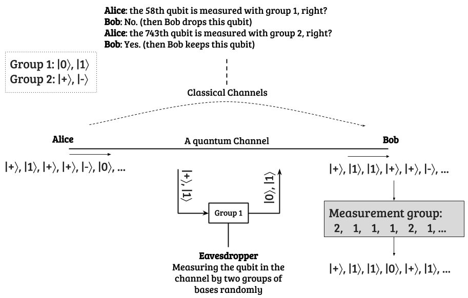
In this protocol, Alice sends a series of qubits to Bob in two groups of bases. Each basis in group 1 is not orthogonal
to each basis in group 2.
Group 1: |0⟩and|1⟩
Group 2: |+⟩and|-⟩
where |+⟩ =  (|0⟩ + |1⟩) and |-⟩ =
  (|0⟩-|1⟩) We can see that in total there are 4 states in two groups of bases.
Alice will randomly choose one state from the 4, with probability all
(|0⟩-|1⟩) We can see that in total there are 4 states in two groups of bases.
Alice will randomly choose one state from the 4, with probability all  , to modulate a photon into corresponding
polarization direction.
, to modulate a photon into corresponding
polarization direction.
Alice will send such photons one by one through a quantum channel to Bob. The quantum channel here can be any
type of physical system discussed before, which can encode a qubit and transmit it. After receiving the qubit, Bob
randomly chooses group 1 or 2 as the bases to measure all the qubit. The quantum channel of lossy so some
photons will be lost in the transmission. So sometimes Bob detects nothing when he measures a
photon.
After Bob’s measurement, Bob will tell Alice all the basis he used in the measurement in public classical channels.
Alice will reply to Bob that which bases Bob used are right. They drop all the qubits processed with inconsistent
bases.
Next, Alice and Bob will share a portion of the states with consistent bases. Here is the critical point,
if there is no eavesdrop, all the results of Bob’s measurement will be the same as the states Alice
used. However, if the qubits are eavesdropped, with large probability, some of the shared states will be
different. The probability could be arbitrarily close to 1 with the increment of the number of qubits they
transmitted.
Here I will show that at least one of the shared states will be different from a very large possibility if the
transmission is eavesdropped on [Cariolaro15].
Assume that Eve is going to measure the qubits in the midway. As Eve does not know the group of bases used by
Alice, she could only randomly choose a group. So for each qubit, with  possibility, she chooses the right bases, and
the other half is wrong.
possibility, she chooses the right bases, and
the other half is wrong.
If Eve chooses the right bases, the state of the qubit keeps. If she chooses the wrong bases, she will certainly change
the state of the qubit. Bob measures the qubit, whose state has been changed, and he will have  possibility
to get the inconsistent state as Alice. Here are all the circumstances where Eve chooses the wrong
bases.
possibility
to get the inconsistent state as Alice. Here are all the circumstances where Eve chooses the wrong
bases.
Table. 4: BB84 Eavesdropper detection
| Alice sends | After Eve measures | After Bob measures |
| |0⟩ | |+⟩ | |0⟩ |
| |0⟩ | |+⟩ | |1⟩ |
| |0⟩ | |-⟩ | |0⟩ |
| |0⟩ | |-⟩ | |1⟩ |
| |1⟩ | |+⟩ | |0⟩ |
| |1⟩ | |+⟩ | |1⟩ |
| |1⟩ | |-⟩ | |0⟩ |
| |1⟩ | |-⟩ | |1⟩ |
| |+⟩ | |0⟩ | |+⟩ |
| |+⟩ | |0⟩ | |-⟩ |
| |+⟩ | |1⟩ | |+⟩ |
| |+⟩ | |1⟩ | |-⟩ |
| |-⟩ | |0⟩ | |+⟩ |
| |-⟩ | |0⟩ | |-⟩ |
| |-⟩ | |1⟩ | |+⟩ |
| |-⟩ | |1⟩ | |-⟩ |
So for each qubit shared by Alice and Bob publicly, with the possibility  , the measurement result of Bob will be
different from the state sent by Alice. If there are n qubits that are eavesdropped on, the possibility that all of them
are consistent is (1 -
, the measurement result of Bob will be
different from the state sent by Alice. If there are n qubits that are eavesdropped on, the possibility that all of them
are consistent is (1 - )n = (
 )n. This probability could be arbitrarily small. So, in reality, it is impossible that Eve
can eavesdrop without being detected.
)n. This probability could be arbitrarily small. So, in reality, it is impossible that Eve
can eavesdrop without being detected.
If Alice and Bob do not find any adversary, they could use the qubits unreleased in the public channel as the secret key encrypting the messages. BB84 is simple and effective. Many advanced quantum communication experiments use BB84 to test the communication quality.
The early approaches to QKD are based on optical fibers. Even for the ultra-low loss optical fibers, the attenuation
coefficient is 0.2 dB/km. Usually, people need to insert a quantum repeater, which is used to recover corrupted
quantum states, about every 60 km in the midway of the quantum channels. However, because of the Nocloning
theorem, a state cannot be amplified without any noise. So the optical-fiber-based QKD can only transmit quantum
states for hundreds of kilometers.
A team developed satellite-based QKD that can overcome the disadvantages of optical fibers [Liao17]. They use a
green laser (λ = 532 nm) to transmit photons between a ground station and a satellite in a sun-synchronous orbit.
They tested BB84 protocol on such a system and achieved a kilohertz key rate, which means that such a system
could transmit thousands of qubits per second, over more than one thousand kilometers. Such a key rate achieved
by using satellite is about 1020 times higher than the key rate we can reach with optical fibers in the
same length. This QKD approach has the potential to be used to build an intercontinental quantum
network.
However, the traditional satellite-based QKD experiments are conducted when the satellites are covered by the
shadow of the earth in order to avoid being influenced by the sunlight, which is a strong noise source. Another team
achieved long-distance free-space QKD in daylight by changing the working wavelength and photon detectors
[Liao17a]. According to the radiation spectrum of the sun, the power of sunlight is stronger at 800 nm than 1550
nm. So the team selected 1550 nm as the working wavelength. In such wavelength, the Rayleigh scattering is only
7% of it in 800 nm, which dramatically increases the signal-to-noise ratio. They developed a new single-photon
detector whose total detection efficiency is 8% under 200 mW pump power. The team transmitted
standard BB84 bases with a key rate from 20 to 400 bits per second from one to the other side of a
natural lake over 53 km. The total channel loss is 48 dB in local time from 15:30 to 17:00 on sunny
days.
Such a result gives us confidence in inter-satellite quantum communication in daylight. As we know that
geosynchronous orbit satellites are in the sunlight zone with a probability of about 99%, the daylight quantum QKD
will improve the efficiency of the geosynchronous orbit satellite significantly.
In this section, we see how the BB84 protocol encrypts classical messages and prevent the qubits from being eavesdropped on. Then two recent works overcoming the disadvantages of optical fibers and night-time quantum communication are introduced. QKD is potentially the most popular encryption approach in the new era. We could also expect a global quantum network based on QKD from the satellites.
This paper shows a new type of communication method based on the quantum phenomenon. Starting with
mathematics fundamental for understanding the representation of a quantum state and its revolution, it shows the
differences between the classical and quantum information theory are presented. The state vectors of
quantum systems can be expressed as unit vectors in Hilbert space. The density matrix is introduced to
express a mixed state and to calculate the quantum entropy of a qubit. Quantum measurement
is one of the most critical concepts of quantum communication because the measurement introduces
uncertainty into a quantum communication system. The uncertainty guarantee that measurement is not
invertible.
We can see that there are many features to which we cannot find analogs in the classical world, for example,
negative conditional quantum entropy. A quantum system could become more uncertain if a part of it is
known. The Nocloning theorem prevents an eavesdropper from coping a qubit and forwarding the original
one.
Next, QT and SDC show two anti-intuitive communication approaches. Actually, the shared entangled pair of qubits
is the key to these two applications. The entanglement guarantees the relationship between two distant qubits so a
state could be ”transported” based on such relationship. In terms of physics, no information could be transmitted
by operating an entangled pair because if so the information will have a speed exceeding the light speed. For SDC,
in total there are 2 qubits sent, so the overall efficiency of transmission is the same as the classical channel. But with
quantum entangled pair, a qubit could be encoded even after it has been sent out! This is the most amazing part of
SDC.
Finally, QKD is described with its most famous BB84 protocol. From that example, it is shown that if the number
of qubits sent is large enough, it is impossible to keep the state unchanged after measurement. In
other words, any eavesdropping will definitely be detected. QKD also needs the assistant of classical
channel.
In the end, we see that satellite-based daytime QKD is gradually becoming a reality. Sending qubits from satellite to ground and between satellite is exciting technology because it avoids the optical loss of optical fiber. The satellite link will become the most applicable implementation of QKD.
[Wilde13] M. Wilde, “Quantum information theory,” Cambridge University Press, 2013, ISBN: 9781107067844
[Carnal91] O.Carnal and J. Mlynek, “Young’s double-slit experiment with atoms: A simple atom interferometer,” Physical review letters, 66(21), 1991, 2689 pp., https://journals.aps.org/prl/abstract/10.1103/PhysRevLett.66.2689
[Pathak13] A. Pathak, “Elements of quantum computation and quantum communication,” CRC Press, 2013, ISBN: 978-1466517912
[Bennett84] C. Bennett and G. Brassard, “Quantum cryptography: Qublic Key Distribution and Coin Tossing,” In Proceedings of the International Conference on Computers, Systems and Signal Processing, 1984, https://cyberleninka.org/article/n/903792.pdf
[Liao17] S. Liao, W. Cai, W. Liu, L. Zhang, Y. Li, J. Ren, J. Yin, et al, “Satellite-to-ground quantum key distribution,” Nature 549, no. 7670, 2017, 43 pp., https://arxiv.org/ftp/arxiv/papers/1707/1707.00542.pdf
[Liao17a] S. Liao, H. Yong, C. Liu, G. Shentu, D. Li, Jin Lin, H. Dai, et al, “Long-distance free-space quantum key distribution in daylight towards inter-satellite communication,” Nature Photonics 11, no. 8, 2017, 509 pp., https://sias.ustc.edu.cn/_upload/article/files/63/ae/36f6b0bd498595eb46eb5b6390b4/023b6b24-4045-4684-a494-b69b72bbf664.pdf
[Lucamarini18] M. Lucamarini, Z. L. Yuan, J. F. Dynes, and A. J. Shields, “Overcoming the rate–distance limit of quantum key distribution without quantum repeaters,” Nature 557, no. 7705, 2018, 400 pp., https://www.nature.com/articles/s41586-018-0066-6
[King77] D. S. King, P. K. Schenck, K. C. Smyth, and J. C. Travis, “Direct calibration of laser wavelength and bandwidth using the optogalvanic effect in hollow cathode lamps,” Applied optics 16, no. 10, 1977, 2617-2619 pp., https://www.osapublishing.org/ao/abstract.cfm?uri=ao-16-10-2617
[Cariolaro15] G. Cariolaro, “Quantum communications,” Heidelberg: Springer, 2015, ISBN: 978-3-319-15599-9
[Bennett93] C. H. Bennett, G. Brassard, C. Crepeau, R. Jozsa, A. Peres, and W. K. Wootters, “Teleporting an unknown quantum state via dual classical and Einstein-Podolsky-Rosen channels,” Physical review letters 70, no. 13, 1993, 1895 pp., https://journals.aps.org/prl/pdf/10.1103/PhysRevLett.70.1895
[Bennett92] C. H Bennett, and S. J. W. “Communication via one-and two-particle operators on Einstein-Podolsky-Rosen states,” Physical review letters 69, no. 20, 1992, 2881 pp., https://journals.aps.org/prl/abstract/10.1103/PhysRevLett.69.2881
[Kaye07] P. Kaye, R. Laflamme, and M. Mosca “An introduction to quantum computing,” Oxford University Press, 2007, ISBN: 978-0198570493
[Shannon48] C. E. Shannon, “A mathematical theory of communication,” Bell system technical journal 27, no. 3, 1948, 379-423 pp., https://pure.mpg.de/rest/items/item_2383162/component/file_2456978/content
[Zhang18] Q. Zhang, F. Xu, Y. A. Chen, C. Z. Peng and J. W. Pan,“ Large scale quantum key distribution: challenges and solutions,” Optics Express, 26(18), 2018, 24260-24273 pp., https://www.osapublishing.org/oe/abstract.cfm?uri=oe-26-18-24260
| CNOT | Controlled-NOT |
| QKD | Quantum Kry Distribution |
| QT | Quantum Teleportation |
| SDC | Superdense Coding |