| Dali Ismail, Steven Harris, dalieismail@gmail.com, sharris22@wustl.edu (A project done under the guidance of Prof. Raj Jain) | Download |
Recently interest in big data has increased due to new developments in the field of Information Technology from the higher network bandwidth, to increases in storage volume, and affordability. One solution to the problem of big data is available from Apache, and is known as Apache Hadoop. In this paper, we will introduce some of the disaster recovery techniques, explain what big data is, explore Hadoop, and its related benchmarks. We will leverage these observations to evaluate the feasibility of a dynamic Hadoop clusters running on physical machine as opposed to virtual systems.
Keyword: Disaster recovery, Big data, Hadoop, Benchmark, Performance analysisIn the field of Information Technology, fault tolerance is requisite for all mission critical systems. One important consideration of fault tolerance is disaster recovery. Having the ability to transfer operations from an operational site to an off-site backup location in response to natural disasters, terroristic threats, or internal disruptive events, can be an arduous task. There are many factors to be taken into consideration including data replication, maintaining identical hardware, as well as business continuity planning decisions such as whether the backup location site will be operated by the organization or contracted to companies specializing in disaster recovery services [Bala13]. Particularly, disaster recovery or more commonly known as backup sites can be segmented into three categories. Those being, cold sites, warm sites, and hot sites.
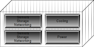
Figure 1: SGI Ice Cube data-center
These containers usually contain all the necessary items such as servers, storage, networking, cooling, and to some extent power as seen in Figure 1. The typical resources allocated to a standard SGI (Ice Cube) compartmentalized data-center can be seen in table 1.
Table 1: Modular Datacenter Resources
| Configuration | Small | Medium | Large |
| Power | < 1MWatt | 1-4 Mwatts | >4 Mwatts |
| Volume | 1440 (ft^3) | 3000(ft^3) | 5643(ft^3) |
| Max MDC | 4 | 4 | 3 |
| Racks per MDC | 4 | 10 | 20 |
| Total Possible Racks | 16 | 40 | 60 |
| Max Load per Rack (KW) | 35 | 22 | 35 |
| Input Power Per MDC (KW) | 148 | 233 | 742 |
| Four-Post Rack Units per MDC | 51 | 51 | 54 |
| Roll-In Rack Max Height | 89.25” | 89.25” | 98 |
| PUE | 1.02 to 1.057 | 1.02 to 1.06 | 1.02 to 1.06 |
| 4-Post Rack Units per MDC | 204 | 510 | 1080 |
| Total Possible 4-Post Rack Units | 816 | 2040 | 3280 |
| Max Cores per MDC | 4896 | 12240 | 24,4880 |
| Max Storage per MDC(PB) | 7.168 | 17.92 | 35.84 |
| Total Possible Cores | 19584 | 48960 | 73440 |
| Total Possible Storage (PB) | 28.672 | 71.68 | 107.52 |
Clearly, the typical SGI container has a configuration that is comparable to other vendors. We observed that this level of hardware and power consumption makes for a rather efficient “datacenter in a box” in you will. However, we have noticed in our research that many of the disaster recovery solutions whether stationary or mobile are ultimately inherently centralized. This is in stark contrast to typical data-center topologies that often extend across cities, states, and countries. Although the physical hardware may be centralized in data centers, the processing and much of the management may be distributed across the range of systems unlike mobile disaster recovery solutions that tend to perform most of the processing and computations on site. The distribution of datacenters across distances allows the management, control, and service planes to be separated from the data, thereby simplifying administration, partitioning, provisioning, and orchestration tasks.
As data-centers have traditionally been used, to allow server farms and server clusters to have dedicated space to coordinate and process large amounts of data, we see this paradigm shifting to virtualized solutions. That is, while continuing to function in the datacenters topology, the developments in computer technology are rapidly shifting to utilized unstructured systems that may not have the same organization as found in the datacenter.
With this paradigm shift, we also see new methods appearing to process larger datasets. The datasets with the largest cardinality are generally referred to as big data. This type of data can be structured, unstructured, loosely correlated, or distinctly disjoint. Current solutions attempt to take these large sets of data, which may be unwieldy and create a more malleable form of big data that may be partitioned across numerous systems. By aggregation of the smaller dataset solutions, the new methods allow finding the solutions to the big data problems.
Typical Big Data is measured by variety, velocity, and volume. These three categories are known in the industry as the “three V's of big data”. As seen in Figure 2, variety can be a disjoint or non-disjoint set of data such as music, video, encryption schemes, or any plethora of data traveling across the Internet [Ivanov13]. Data with variety can be challenging to categorize, as it may not be correlated due to its variability. Velocity on the other hand as the name implies often refers to the speed of the data. There is quite a bit of data that is fixed, such as files on a hard disk, flash drive, or a DVD, are often referred to as batches because it is data that is waiting to be processed and may be processed sequentially or via random access. However, most of the data that proliferates the internet and data centers today tends to be less stationary such as real-time data from sensors, streams of data such as dynamic updates, communications, firewalls, or intrusion detection system messages for instance. Volume refers to the size of the data. This size of big data tends to fluctuate depending on the problem to be assessed [Zikopoulos12].
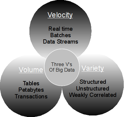
Figure 2: The three Vs of big data
However, the datasets tend to be rather large, such as a database of every employees badge swipe time in a transcontinental corporation, the blood type of every person in North America, or the frequency of Arabic words used across the Internet.
In all cases, Big Data contains at least one element from each sphere. The three V's of big data make it increasingly challenging to process this level of data on a single system. Even if one were to disregard the storage constraints for a single system, and perhaps utilized a storage area network to store the petabytes of incoming data, the bottleneck would be the standalone systems processor. Whether single core or multi-core, all data would have to be processed through a single system that would ultimately take substantially more time than partitioning the data across a large number of systems.
To solve some aforementioned issues dealing with Big Data, the Apache Foundation is helping development of Apache Hadoop. This solution is a Distributed File System designed to run on commodity hardware as well as higher profile hardware. The Hadoop Distributed File System (HDFS) shares many attributes with other distributed file systems [Borthakur07]. However, Hadoop has implemented many features which allow the file system to be significantly more fault tolerant than utilizing typical hardware solutions such as Redundant Array of Inexpensive Disks (RAID) or Data Replication alone [Chang08]. In this section, we will explore some of the reasons Hadoop is considered a viable solution for big data problems
Hadoop provides performance enhancements allowing for high throughput access to application data, as well as streaming access to file system resources, which is becoming increasingly challenging to manipulate for larger datasets, [Borthakur07]. Many of the design considerations can be subdivided into the following categories:
In the most general sense, applications which request computations from nodes which are within some small radius of the application are significantly more efficient and cost effective than computational requests which encompass greater distances, particularly as the size of data sets increases. Requesting computational results closer to applications also decreases network congestion as requests are answered more efficiently. Consequently, the HDFS provides extensions, which allow the applications to relocate themselves to the vicinity of the processing nodes for greater efficiency.
In this topology, hardware failure is simply an unpleasant fact in data processing. Since the HDFS may be partitioned across hundreds if not thousands of devices, with each node storing some portion of the file system, there is a significant probability that some node or component in the HDFS may become non-functional. In those instances, one goal of the HDFS is to provide quick automatic recovery, and reliable fault detections throughout the topology.
All applications utilizing the HDFS tend to have large datasets in ranges from gigabytes to petabytes. The HDFS has been calibrated to adjust to these large volumes of data. By providing substantial aggregated data bandwidth, the HDFS should be able to scale to tens of hundreds of nodes per cluster.
As the applications, which run on the HDFS, are more specialized instead of general purpose, many of these applications require streaming access to the datasets. Therefore, the HDFS is geared more towards batch processing in contrast to interactive processing[Ghemawat03]. This also allows for higher throughput data access instead of the traditional low latency that is often one of the primary goals in traditional general-purpose file systems.
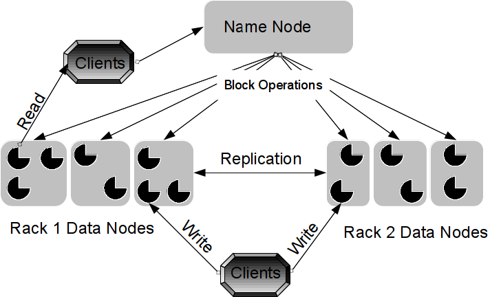
Figure 3: Hadoop Filesystem Topology
The HDFS utilizes master/slave architecture as seen in Figure 3. A typical HDFS cluster contains a Name node, that is, a master server that manages the names and access to the file system by the Data nodes [Garlasu13]. There are typically a number of Data nodes consisting roughly of one per node per cluster that regulates the attached storage of the hardware/virtual devices they run on. The master node exposes the file system namespace and enables Data nodes to store data on the HDFS. Internally, the files are split into blocks that are stored and distributed to the Data nodes within the cluster. The Name node performs operations such as opening, renaming, and closing directories and files in the file system, as well as creating mappings between the Data nodes and data blocks. The Data nodes have a similar function but their operations refer to blocks. In that respect, they are responsible for the creation, replication, and deletion of data blocks when requested by the Name node [White12].
Benchmarks are the standard used to compare the performance between systems to differentiate between possible alternatives. In terms of Big Data, performance is an integral part of storage and retrieval within Hadoop.
When setting up a Hadoop cluster we would like to know if a cluster is correctly configure and this can accomplish by running a tasks and checking the results [White12]. In order to measure the performance of our cluster, our best choice would be to isolate a cluster and execute benchmarks so we can determine the resources utilization and the cluster processing speed.
This section explore the benchmarks used to test the performance of Hadoop clusters, some of the benchmarks listed are used to test Hadoop cluster performance in real world scenarios. Hadoop contains many benchmarks packages encapsulated in Java Archive JAR files [White12] as follows:
Performance is critical when discussing Hadoop clusters. These clusters may run on bare-metal, virtualized environment or both. A performance analysis of individual clusters in each environment may determine the best alternative to obtain the expected performance. In this section, we explore the setup of our clusters, what factors affect Hadoop and the results of our test.
After reviewing numerous scenarios for feasible disaster recovery solutions, we would like to leverage some of the fundamental paradigms of disaster recovery to develop some measure of performance agility in Big Data solutions. As we have mentioned previously many of the disaster recovery solutions are stationary. We have endeavored to develop a Big Data topology that incorporates balance, speed, and endurance. Most solutions in big data are installed either on physical systems or in virtual machines. We have developed an implementation of a Hadoop map reduce cluster that runs entirely in memory. This will allow us to obtain significant performance benefits, as the input/output (I/O) throughput of random access memory (RAM) is inherently faster than conventional systems. We utilized four Intel eight Core i7-2600 3.4 GHz servers with eight gigabytes (GB) of ram for physical clusters. For the four virtual machines, we utilized four 2 GHz Intel Core i7 server with eight GBs of ram. We executed the TestDFSIO benchmarks on these systems to give us data to compare and contrast the feasibility of a dynamic Hadoop cluster on commodity hardware.
Different factors may affect the performance of the cluster; some of those factors may reside in the Hadoop architecture while the others may be external factors. Table 2 lists some of the factors affecting Hadoop cluster performance [White12].
Table 2: factors affecting Hadoop cluster performance
| Performance optimization parameters | External factors |
| Number of maps | Environment |
| Number of reducers | Number of cores |
| Combiner | Memory size |
| Custom serialization | The Network |
| Shuffle tweaks | |
| Intermediate compression |
Hadoop internal factors (also called parameters) can be set by the user on demand to optimize the performance of the cluster.
In our Hadoop cluster experiments, we will study the environment (Physical and Virtual); particularly the environment where Hadoop cluster runs will be the primary factor on performance due to the overhead of virtualization on the system performance.
In this test, we are running two data nodes and one name node on different system utilizing a hypervisor. We used 10x the number of slaves for the number of maps as well as 2x the number of slave for reducer. We executed the TestDFSIO benchmark to test the I/O performance of HDFS, and the response variable in this experiment was the elapse time (in seconds). The results, which follow after presented after applying logarithmic transformations to reflect the variety of the data [Jain91]:
Table 3: Benchmark elapse time
| Benchmark | Physical | Virtual | ||
| 2 nodes | 4 nodes | 2 nodes | 4 nodes | |
| TestDFSIO write | (16, 13, 13) | (16, 16,15) | (61, 79, 51) | (139, 215, 241) |
| TestDFSIO read | (13, 13, 13) | (13, 14, 14) | (27, 27, 24) | (58, 47, 61) |
In our experiment we analyzed the results using the (2^3)*3 factorial design to determine the effects of factors under study on the cluster performance, Y is the average of the elapse time from table 3 [Jain91].
A: the environment effect
B: workload
C: number of nodes
Table 4: analysis of (2^3)*3 design
| Effects | Measured response | ||||||||
| I | A | B | C | AB | AC | BC | ABC | Y | |
| 1 | -1 | -1 | -1 | 1 | 1 | 1 | -1 | 1.14 | |
| 1 | 1 | -1 | -1 | -1 | -1 | 1 | 1 | 1.79 | |
| 1 | -1 | 1 | -1 | -1 | 1 | -1 | 1 | 1.11 | |
| 1 | 1 | 1 | -1 | 1 | -1 | -1 | -1 | 1.413 | |
| 1 | -1 | -1 | 1 | 1 | -1 | -1 | 1 | 1.19 | |
| 1 | 1 | -1 | 1 | -1 | 1 | -1 | -1 | 2.283 | |
| 1 | -1 | 1 | 1 | -1 | -1 | 1 | -1 | 1.13 | |
| 1 | 1 | 1 | 1 | 1 | 1 | 1 | 1 | 1.736 | |
| Total | 11.79 | 2.65 | -1.01 | 0.88 | -0.83 | 0.74 | -0.2 | -0.14 | |
| Effect(Total/8) | 1.47 | 0.33 | -0.12 | 0.11 | -0.10 | 0.09 | -0.02 | -0.01 |
Table 4 shows the effects of each factor and factors interaction at the effect row.
Next we calculated the errors in our model as shown in table 5:
Table 5: model errors
| Estimated Response | Errors | ||
| E1 | E2 | E3 | |
| 1.14 | 0.06 | -0.03 | -0.03 |
| 1.79 | -0.01 | 0.1 | -0.09 |
| 1.11 | 0 | 0 | 0 |
| 1.413 | 0.016666667 | 0.016666667 | -0.03333333 |
| 1.19 | 0.01 | 0.01 | 0.02 |
| 2.283 | -0.143333333 | 0.046666667 | 0.096666667 |
| 1.13 | -0.02 | 0.01 | 0.01 |
| 1.736 | 0.023333333 | -0.066666667 | 0.043333333 |
The sum of model errors should equal zero, because errors are the difference between measured response and estimated response [Jain91]. After calculating the errors we calculate the allocation of variation to estimate the effect of each factor in our experiment. The results are shown in table 6.
Table 6: Allocation of Variation
| SSY | 56.0332 | ||
| SS0 | 52.15601667 | ||
| SSA | 2.640066667 | 68% | The environment is the main factor affecting the performance |
| SSB | 0.385066667 | 9% | 9% of the performance affected by the workload |
| SSC | 0.294816667 | 7% | 7% affected by the number of nodes |
| SSAB | 0.260416667 | 6% | |
| SSAC | 0.209066667 | 5% | |
| SSBC | 0.015 | 0.3% | Effect is negligible |
| SSABC | 0.00735 | 0.7% | Effect is negligible |
| SSE | 0.0654 | 1.6% | Errors in the model affecting the performance are small percentage |
Next we calculated the confidence interval for the effects to make sure our calculation is significant. We selected the value 1.746 from the t-value table for 90% confidence interval and the results are shown in table 7 below [Jain91].
Table 7: confidence intervals of the Q effects
| Effect | Confidence Intervals | |
| q0 | 1.454166667 | 1.494166667 |
| qA | 0.311666667 | 0.351666667 |
| qB | -0.146666667 | -0.106666667 |
| qC | 0.090833333 | 0.130833333 |
| qAB | -0.124166667 | -0.084166667 |
| qAC | 0.073333333 | 0.113333333 |
| qBC | -0.045 | -0.005 |
| qABC | -0.0375 | 0.0025 |
All affect are statically significant except the interaction between A, B and C effect because it includes zero. Finally, we will use the virtual test to validate our model and we will assume that errors are statically independent and normally distributed [Jain91].
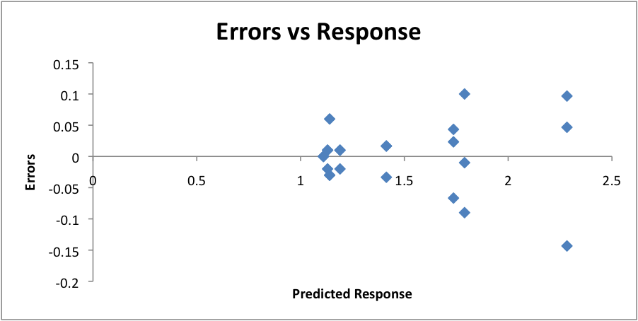
Figure 4: Errors vs. Response
In figure 4 it’s hard to tell if there is a pattern in the chart, which means errors are independent.
To check if the errors were normally distributed we created Q-Q plot to verify that, as shown in figure 5
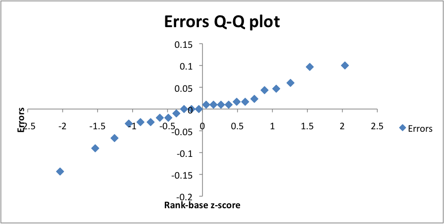
Figure 5: Q-Q plot of errors
From figure 5 we can observe that errors are normally distributed and from both figure 4 and 5 we can say that our experiment results reflect the real performance of our system.
After analyzing the results of our experiment, calculate the errors in the model; calculate the allocating of variation and the confidence intervals for the effects we can say with confidence that the environment is the main factor that affect the performance.
In our experiment we found that Hadoop cluster running in virtual environment is significantly perform low than the one running is physical environment (physical machine), and other factor might affect the performance but in our study we focused on the environment effect which is 68% affecting the performance of the Hadoop cluster.
We prepared a comparison chart between the performances of the Hadoop cluster in both environments. Figure 6 represents the performance difference between the clusters running in different environments.
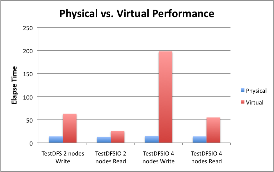
Figure 6: Performance comparison
From these results, we observe that Hadoop performance, confirmed that the virtual Hadoop cluster performance is significantly lower than the cluster running on physical machine due to the overhead of the virtualization on the CPU of the physical host. The factors, which affect the performance (RAM size, network bandwidth), were considered in our experiment. However, our study was directed towards the effect of environmental factors on the performance.
During the course of our investigation, we have explored some of the solutions to problems such Disaster Recovery, Big Data processing, and Distributed File Systems. After looking at those solutions, we developed a means to leverage the benefits of each category and created a dynamic Hadoop cluster that operates entirely in Random Access Memory. We found that the commodity systems, while both antiquated and less responsive performed significantly better using our implementation than standard Virtual Machine implementations utilizing standard hypervisors.