| Adam Drescher, adrescher (at) wustl.edu (A paper written under the guidance of Prof. Raj Jain) |
Download |
Virtual machine allocation is an interesting topic at the intersection of a few different disciplines. Additionally, industry and academia are both pursuing the field of study. We are recently adding virtual machines to our Open Networking Laboratory at Washington University in St. Louis. This laboratory needs to ensure a certain amount of experimental isolation between networking experiments running on the same hardware. We want to know how many virtual machines we can add onto a host machine until it degrades the networking performance. From the results of our paper, we recommend a maximum of five virtual machines, each with 2 CPU cores and 4GB of RAM, to be allocated on a host machine with 24 cores and 64 GB of RAM. Going above this threshold will quickly degrade the performance of UDP transfers among the virtual machines.
| Acronym | Definition |
|---|---|
| ANOVA | Analysis of Variance |
| CPU | Central Processing Unit |
| FIFO | First In, First Out |
| gbps | gigabits per second |
| IP | Internet Protocol |
| mbps | megabits per second |
| MAC | Media Access Control |
| MTU | Maximum Transmission Unit |
| NIC | Network Interface Card |
| ONL | Open Networking Laboratory |
| RAM | Random Access Memory |
| TCP | Transmission Control Protocol |
| UDP | User Datagram Protocol |
| VM | Virtual Machine |
Virtual Machine allocation is a problem that has the attention of both industry and academia. The crux is knowing how to provision the tenant machines in relation to the host machines. There can be tenants of a variety of sizes. Some may have strict latency requirements, whereas others may not. Depending on the load of a particular host machine, we might have room for another tenant. On the other hand, how much is too much? These are some of the motivating questions and concerns for the general area of virtual machine allocation.
As we will see, virtual machine allocation is currently an interesting problem domain. Industry has focused much money and time on the problem. Unfortunately, yet understandably, they do not discuss their solutions; we have little to no insight how Amazon or VMWare solve their virtual machine allocation problems. Academia is more open with their results. However, academia works on problems that are more complex than what we aim to study. They frequently use migration and other techniques that are a bit heavy handed for our laboratory setting, at least preliminarily. Our pursuits are much more narrow. We do not need virtual machine migration for our preliminary study. Our motivating question is simply how many virtual machines can we put on a host machine until it degrades the networking performance to an unsatisfactory level. This is a real problem for a real laboratory, so while it is a simpler problem it is necessary to pursue.
In this paper, we will perform a performance analysis study on virtual machine allocation in the Open Networking Laboratory, a networking laboratory that is run by our research group at Washington University in St. Louis. Section 2 offers a primer on the networking in general and how the Linux kernel performs common networking tasks. Additionally it explains the Open Networking Laboratory, which motivate both the study as a whole and the specific experimental setting. In Section 3, we will discuss the swathe of related work. Specifically, we focus on how well the work relates to our problem, and we mention wisdom imparted on us in the process. The reader should get a broad sense of the state of the art from this section, and also agree that our problem is less complex. In Section 4, we will discuss the exploration performed to motivate our experimental design, i.e. figure out what factors and levels to study at all. Because this is a real systems experiment, it is not clear initially how the many pieces will fit together, and what pieces are important to study. This inquiry is done informally, to lay the groundwork for the formal experimental design and analysis. It is simply to gather intuition for what experiments to design. This led us to create two separate experiments, which are covered in Sections 5 and 6. Section 5 describes the experimental design and analysis of our TCP experiment in a networked setting, and Section 6 describes the design and analysis of our UDP experiment in the same setting. We separated these two studies because TCP and UDP have different properties and factors, and joining them in one study would be clunky. Lastly, Section 7 summarizes the results of our paper.
Networking is not accomplished through one homogeneous protocol. Rather, it is accomplished by a layered approach, where different protocols are built on top of each other. Each layer performs a specific function. At most of the layers, there are different protocols that can be used without affecting the operation of the rest of the networking stack. A summary of the layers, adapted from [Kurose13, Wyllys01] is given below in Table 1. For our experiment we particularly care about layers 2 through 4, so they are highlighted in the table.
| Layer | |||
|---|---|---|---|
| Number | Name | Protocols of Interest | Function |
| 5 | Application | Provides services to users and programs | |
| 4 | Transport | TCP, UDP | Transfers data between end systems |
| 3 | Network | IP | Routes data, logical addressing |
| 2 | Data Link | Ethernet | Physical addressing, Channel access control |
| 1 | Physical | Receiving and transmitting electric signals | |
The Network Interface Card (NIC), which is the hardware that allows are computers to communicate over a medium like a wire, operates on layers 1 and 2. The NIC receives Ethernet frames and passes it on to the layers above. Each NIC has a corresponding hardware address that all layer 2 protocols rely on. These are called MAC addresses and are a series of hexadecimal digits of the form fe:0c:0c:09:00:00. These hardware addresses are required to talk to machines we are directly connected with, whether via a physical cable or wireless media. Additionally, each NIC has a network interface name that can be used to display various statistics or control the state of the NIC.
Next we have layer 3, which is the IP layer of the protocol stack. IP is known as the slim waist of the Internet [Tanenbaum11], because essentially every networking technology at a higher or lower level uses it for its layer 3 protocol. Layer 3 uses IP addresses, e.g., 192.168.1.1, which are a logical address used for routing across multiple hops in a network. IP routes traffic over a sequence of physical connections in order to deliver the traffic to its logical destination.
Lastly, layer 4 has two dominant protocols that are used for data transport: TCP and UDP. TCP and UDP are opposites in many respects. TCP provides a mechanism for reliable data transport and guarantees in order delivery. Logically, it establishes a connection that is maintained throughout the duration of the transfer, i.e. it is connection oriented. This means it has mechanisms for keeping track of which packets were successfully received, and adapting the sending rate so that the protocol does not overwhelm the available networking resources. The latter of the two mechanisms is called congestion control. There are a variety of different strategies for performing each of these mechanisms, and as a result there are a variety of TCP algorithms available that can be used. UDP on the other hand is connection less. Anything that is addressed to a valid IP-port combination will be happily accepted. There is no guarantee for in order delivery or reliable data transfer. Additionally, it sends as fast as the bottleneck link can allow. It is easy to see that these two protocols are considered orthogonal. Now that we are refamiliarized with the details of networking, we can move on to some more specific details.
There are a few more low level details we need to discuss before we can move on. Because the machines in the Open Networking Laboratory are Linux machines, we need to understand how Linux networking works to fully understand our evaluation. We will use the following figure as a reference for this section [Roscoe12]:
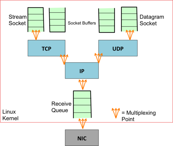
We can see that when an Ethernet frame arrives at the NIC, it is passed to the Linux kernel. To pass the received Ethernet frame into the kernel, the NIC generates a high priority software interrupt to notify the kernel it has a frame to pass on [Roscoe12]. When the interrupt is generated, a device driver needs to handle the interrupt, and will pull the frame into the receive queue. Smarter schemes can be used, but one-at-a-time is the simplest to understand. It is important to note that standard Ethernet frames have a maximum length of 1522 bytes [Horton08]. An IP packet that is larger than 1522 bytes will be fragmented into smaller pieces before it can be sent over Ethernet. The IP layer will perform this fragmentation on sending, and also reassembly into the larger packet on receiving. This increases overhead because reassembling many fragments into a larger IP packet takes time, and under certain conditions can be difficult to do at link rate without making reassembly errors. When this happens, the entire large IP packet is lost, not just one of the smaller Ethernet frames. As the packet passes through the IP part of the stack, after it has been reassembled it can then be passed on to the UDP or TCP part of the stack [Benvenuti06]. If it is a TCP flow, it will be parsed and enqueued in the appropriate stream socket, which is simply a socket than supports TCP connections. If it is a UDP flow, it is parsed and enqueued in the appropriate datagram socket. That means each socket has their own socket buffer. Socket buffers and the transmit and receive queues, denoted TX and RX respectively, have a finite size, which means when they are full they are forced to drop any other incoming packets. Because of this finite capacity, these buffers and queues are specifically called FIFO queues, circular buffers, or ring buffers. Additionally, any of the points we have to demultiplex at will require sharing the packet handling resources. These are all areas where packet loss can manifest itself, and should be carefully monitored. These are sufficient details to be able to pin down packet loss.
The computer science department at Washington University in St. Louis has a research lab called the Applied Research Laboratory, of which I am a member. This research lab runs the Open Networking Laboratory (ONL), which is a networking laboratory available to anyone in the world with a network connection and a valid reason to use the laboratory. ONL consists of many host machines of a variety of different cores, many routing clusters, and software routers. The motivation behind ONL is that most networking experiments are performed by simulation, e.g., mininet, as opposed to run on the real hardware [Wiseman08]. Simulation can only go so far — it is often preferred to be able test networking protocols on real hardware, whether it be for performance or complex interactions that would be difficult to mimic in a simulation. Users can design and reserve experimental topologies with the variety of machines that ONL provides. Once they are allocated their topology, the user has a way to run real networking experiments on real machines. It is absolutely key that different user's experiments do not influence each other's results and experimental isolation is preserved. This is necessary when requiring precise numbers for reliable results. Additionally, the current ONL provides a logical 1 gbps link between all hosts.
Recently, we have been adding virtual machines to ONL, so users can install whatever software they want to run their experiments. This makes both experimental isolation and bandwidth guarantees more interesting problems. Before, experiments would reserve whole physical machines, and those would be on their private virtual local area network. However, in the tenant / host machine setting in virtual environments, now virtual machines from two (or more) different experiments can be running on the same physical host machine. This means we will need to be careful about ensuring separation of resources, since the virtual machines will both be using CPU cores, RAM, and bandwidth on the same machine. Additionally, it is generally known that virtual machine networking is slower [Rizzo13, Menon05]. In fact, we are not sure if we can provide the same guarantees that we provided in the physical host scenario; it is possible that the additional limitations of the virtual environment means by nature the results are less precise, and that is how known up front.
Industry and academia are working on the virtual machine allocation problem from two different perspectives. Additionally, both are solving harder problems than what we have in mind. As a result, there is not much literature that is directly applicable to our problem (at least not for the stage we are at). However, we should know the state of the art before we proceed.
Many of the academic papers focus on cloud computing environments. These provide various algorithms for the best virtual machine allocation in cloud environments. Marjan Gusev et al. publish an algorithm that gives them optimal resource allocation, i.e., the best distribution of jobs across the possible machines [Gusev12]. Additionally, a variety of other papers also propose solutions for this problem [Xiao13, Yanagisawa13, Stillwell12]. However, all of these solutions leverage migrations. Migrations require migrating all of the virtual machines state on the fly to a new tenant VM on a new host machine, and switching its execution over to the new tenant VM. This is a problem which we do not need to consider, or at least not early on. Additionally, we do not need to be optimal with our resources because we are not operating on a massive scale. As opposed to cloud computing environments, if an easier solution exists it suffices for us to be "good enough". Many of the other perspectives of academia focus on migration specifically [Yao13] or energy aware scheduling. Again, these are bit too heavy handed for us.
Industry seems to be more pragmatic in their approach. Many of the big virtualization companies have documents publishing their recommended configurations when using their specific product. Indeed, these are particular to the virtual machine products that each company offers. However, they provide general guidelines which can be compared against each other, hopefully to the point of gaining previously unknown insight. One thing common to Cisco, VMWare, HP and Microsoft is that they embrace virtualization not just at the machine level but at the network level. To be specific, each of the companies provides virtual switches with their virtual machine server technology. Microsoft uses its Hyper-V switch to perform a variety of security measures, traffic shaping, and experimental isolation. As far as tenant machine resources are concerned, they use a pooling system with guarantees when necessary and sharing unused resources otherwise [Microsoft12]. They do not give any information elaborating on the minimum resources a virtual machine should need for their most recent Windows Server. VMware provides a similar level of detail and similar mechanisms [VMware]. Cisco is a bit more informative with their materials. They require that the minimum dimensions of a single virtual machine be 2 CPUs, 6 GB of RAM, and 132 GB of disk space [Cisco12]. This seems reasonable on the CPU side, but quite heavy on the memory and disk space required. HP was the most informative of the companies; they give distinct advantages and disadvantages of the virtualized networking approach to virtual machines. The most important of these takeaways is a disadvantage of using a virtual switch: virtual switches "consume valuable CPU and memory bandwidth" [HP11]. This will be helpful to keep in mind as we are running our networking experiments. A wealth of information is available in the form of a variety of OpenStack system administration guides [OpenStack14]. They are often quite specific to the details of OpenStack itself. However, it is evident that OpenStack is intended for large operations, i.e. a 6-12 core machine being considered "small". Lastly, Rob McShinsky penned an excellent post on practical virtual machine allocation, which was quite helpful for our initial ideas [McShinsky09]. We have at least gleaned some useful information by knowing the state of industry, and can also look towards the future with more academic pursuits.
We want to ensure virtual machines can retain the same networking performance as physical hosts. Particularly, we want to stress the networking and CPU of the physical hosts by having as many virtual machines on the physical machine as possible. Our maximum configuration will be the minimum between two concerns. First is the distribution of the CPUs and memory to the virtual machines: we want to ensure that there are enough resources dedicated to the physical machine that it can deal with the virtual machines efficiently, and not be over provisioned. Particularly, the physical machines that we will be allocating the virtual machines on have 24 cores and 64 GB of RAM. Right now, our preconfigured VM size is 2 cores and 4 GB of RAM. If we want to leave a core or two to the physical machine for extra tasks, our natural upper bound is 11 VMs due to the number of cores available.
Because ONL is a platform for network testing, these CPU and memory concerns can still be realized through just network testing. If the networking works fine, then the CPU and memory is fine for the purposes of the laboratory. However, we also need to explicitly think about how ONL distributes networking resources. All of the clients and servers will be communicating over a 10 gbps link. However, due to the experimental guarantees of ONL, any one client / server pair should be able to attain 1 gbps. As a result, our natural limitation due to bandwidth will be 10 virtual machines. This is the smaller of the two, and our maximum configuration a user can attain.
The two primary protocols used for our networking experiments are TCP and UDP. As mentioned earlier, these are two ubiquitous transport layer protocols for the Internet. However, TCP and UDP are good at testing and measuring different things. TCP is good for measuring throughput, and due to its congestion control policies the fairness between multiple connections. UDP is less about being fair, and will just send as fast as possible. However, we want to keep the loss rate low, otherwise there is no point in us sending so fast. TCP does not even have loss rate since it guarantees reliability and in-order deliveries to the application layer. It is clear that TCP and UDP have very different response variables and factors, and thus should be two separate experiments.
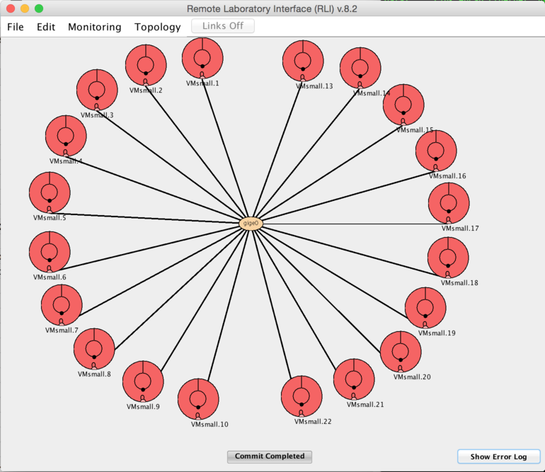
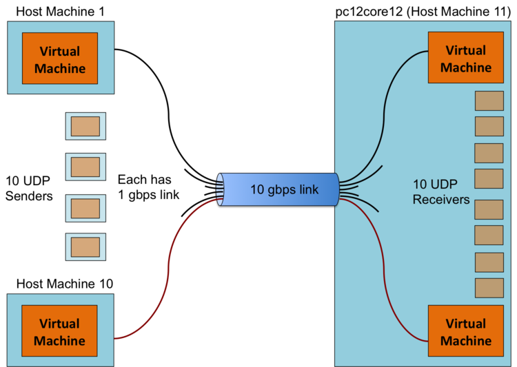
As pictured above, we have a star topology for our experiment. However, the virtual machines on the left half of the diagram are all on different host machines. These machines act as the clients. The virtual machines on the right half of the diagram are all on the same host machine (named pc12core12), so they are sharing their host machines resources between each of the tenant VMs. These machines act as the server, because in general being receiving demands more resources than sending. Each client machine will pick its own unique server to send to, i.e. there will be ten unique flows going to the same physical machine. Ideally, each of these flows will be 1 gbps, and they will unite to deliver a full 10 gbps to the host machine. In the interest of clarity, the logical diagram of our experiment is pictured below.
We are going to test if the host machine can handle all of the receiving VMs transferring at full capacity. In other words, we will test receiving TCP and UDP streams up to our maximum user configuration (10 VMs). Iperf3 is used as our traffic generation tool. It is a recent remaking of the classic iperf utility, which was the standard for networking testing for many years. Iperf3 will allow us to send TCP and UDP streams to a server at whatever rate the link can support.
Theoretically, it is possible that we will run our maximum configuration and the TCP and UDP performance will be just as good as the minimum configuration (one client/server traffic flow). That would be a bit too good to be true, but before we design experiments, we should check to make sure we are not already done. Additionally, some exploration will hopefully help guide us to which factors we should formally study. For TCP there is obviously no packet loss (TCP provides reliable transport). We simply need to compare the baseline throughput to the maximum configuration case. The default settings for the TCP test are a 12KB socket buffer and 10 second test length. Following the transient removal technique from the book, we decided to run the test for 12 seconds and omit the first two seconds from the results [Jain91]. This allows us to skip past TCP slow start and evaluate it when the congestion window is already large. With these settings for TCP, the baseline configuration (one client sending to one server) achieved the full 1 gbps. The maximum configuration (10 flows) was decently close to getting 1 gbps for each of the 10 flows. However, it still had room to improve, so further testing should be done to highlight this. Trying 9 flows would likely be sufficient. Additionally, one or two of the flows typically had lower performance than the rest of the flows in the group. This leads us to believe that a different congestion control algorithm might alleviate that issue. Thanks to Gamage et al. we know that the virtual machine actually sets the TCP congestion algorithm and not the host machine they are tenants of [Gamage11]. As a result, congestion control will be a factor in our formal study. Additionally, the congestion control algorithm will likely level out more if the experiment time is longer, so the time will be a factor as well. We pursued smaller packet lengths, by constraining the MTU or the socket buffer, but iperf3 has a bug where the length will reset to the maximum size segment after a loss or retransmission event occurs. From our initial exploration, it is clear that a \(2^3\) full factorial analysis would be appropriate.
UDP exploration was a bit less straightforward, and more necessary to explore the potential experimental designs. With UDP smaller packet sizes did work, so that is an avenue we will explore. We should establish our baseline with a variety of packet sizes. The bandwidth specified will be 1 gbps, as that is what we would prefer to send at for each flow. The default test time was 10 seconds. We first start with a one flow test, keeping the default socket buffer length / packet length (8KB). Because this is larger than the Ethernet MTU, we will need to fragment and defragment the packet at their respective IP layers in the networking stack.
We see that we have packet loss, but it is not bad at all. However, we should get used to exploring where packet loss occurs.
There are a few things we can notice from our netstat output. First, looking at the IP output we can see there were 907,980 reassemblies required and 151330 packets reassembled successfully. Looking at our iperf3 output above, it reports that we send 151,330 packets. Every packet was fragmented, and it was fragmented into 6 pieces! Note: by simple arithmetic, \(\frac{907,980}{151,330} = 6\). Also, because every packet that required reassembly was successfully reassembled, we can tell that our packet loss did not occur at the IP layer. Next, looking at the UDP output of our netstat command shows that we have 19 "packet receive errors". Because we run this netstat command on our receiving virtual machine, this means that the UDP socket buffer on the virtual machine was full and could not accept 19 incoming packets throughout the course of the transfer.
Next, we want to explore running transfers with a few different packet lengths. First we will run a test with a 1400 byte packet, which is a large packet but will not need to be fragmented or reassembled since it is under the 1522 bytes of the Ethernet MTU. Summarizing the results, there are a few noticeable differences. The first is that we sent 884,545 datagrams for the same length transfer; this is way more than before. However, this is perfectly natural, as we are manually splitting our larger packets into roughly 6 smaller ones, as opposed to forcing the IP layer to fragment and reassemble them. Another noticeable result is that our loss rate went up (to 0.068%). Particularly interesting is that this is not an increase by a rough factor of 6, but much larger. This increased amount of lost packets is due to the same effect: we simply have a larger amount of socket buffer errors. With the smaller packet sizes, the socket buffer is getting strained a little bit more due to the additional overhead from parsing more packet headers.
Next we tried the same setup as we have been using, but with a minimum length UDP packet. The minimum Ethernet frame is 64 bytes. Subtracting away 18 bytes for the Ethernet header and trailer, 20 bytes for the no-options IP header, and 8 for the UDP header, this leaves 18 bytes for our minimum size UDP payload. Using 18 byte payloads, we end up sending 1,503,227 datagrams and losing 57% of them. Again, we have an increase in socket buffer errors from the last time, but it does not account for even close to the 855,115 packets lost in the transfer. To attempt to isolate where packets have been lost, we first check the sending VM and ensure it has no drops or socket buffer errors. As far as the VM is concerned, it sent 1,503,248 packets which is remarkably close to what iperf3 reported as sent. Now we look at the virtual interface on the physical machine and it agrees with our assessment. However, the data interface on the physical machine that the virtual interface feeds into only reports sending 661,718 packets. Mysteriously we lose around 842,000 of our packets in between the virtual interface and the physical data interface; the only entity in between these interfaces is a Linux bridge. This mysterious bug was unresolved over the time of testing. Because we are not able to reliably perform minimum packet size testing, and the difference between 1400 byte socket buffers and 8KB socket buffers is negligible, we will use the default socket buffer size / packet length and not consider it as a factor. As a result, we should just focus on the number of parallel flows until the quality degrades too much to be used.
For our study of the TCP performance of our setup, we designed a \(2^3 5\) experiment. This means we have three factors, each with two levels, and each of these different configurations was replicated 5 times [Jain91]. Our first factor is the TCP congestion control algorithm used for the transfer. The hope is that different TCP algorithms would more fairly spread the bandwidth between the \(N\) flows, so we do not have some flows at ~700 mbps while the others send at close to 1 gbps. The TCP congestion control algorithms we have available are CUBIC and Reno. The second factor is the length of the transfer. We will keep our 10 second test, and compare it with 120 seconds. The goal with the longer transfer time is that the flows will settle into less varied sending patterns, and have converged on a more fair sharing of bandwidth. The last factor being the number of parallel flows. We know from the previous section that 10 flows did pretty well, so we want to see how 9 goes. Our response variables will be throughput and fairness, which will be specifically calculated by Jain's Fairness Index [Jain91].
| Number of Parallel Flows | Experiment Length (s) | Congestion Control Algorithm | Mean Throughput (Mbps) | Standard Deviation of Throughput | Fairness | Standard Deviation of Fairness |
|---|---|---|---|---|---|---|
| 9 | 10 | Reno | 1020 | 0 | 1 | 0 |
| 9 | 10 | CUBIC | 1020 | 0 | 1 | 0 |
| 9 | 120 | Reno | 1020 | 0 | 1 | 0 |
| 9 | 120 | CUBIC | 1020 | 0 | 1 | 0 |
| 10 | 10 | Reno | 938.8 | 59.9 | 0.989 | 0.001 |
| 10 | 10 | CUBIC | 939.1 | 100.2 | 0.998 | 0.003 |
| 10 | 120 | Reno | 939.1 | 22.5 | 0.996 | 0.0002 |
| 10 | 120 | CUBIC | 939.2 | 37.6 | 0.999 | 0.0003 |
As it turns out, 9 was perfect for every category: 1 gbps mean with 0 standard deviation for every possible combination with 9 parallel flows. As mentioned above the response variables we are interested in are throughput and fairness. Obviously, for the case of 9 parallel flows, the fairness score is 1 and the throughput is 1 gbps; it cannot get better. For any of the tests with 10 flows, the global means were all approximately 940 mbps and the standard deviations were quite low. Even with the the appearance of imbalanced flows, their fairness scores were all approximately 0.98-0.99. Our domain knowledge tells us at this point we don't need a formal analysis of the results. We can tell they are good enough already! The decision making process is: if you want 1 gbps of TCP seemingly high likelihood, allocate 9 hosts. If you don’t mind around 0.930 Gbps per flow, then you can allocate 10.
In this section we will cover the one factor analysis for UDP. Our factor was the number of parallel flows going into pc12core12; equivalently, the number of UDP receivers on the host machine. Again, we did five replications per result. We use the default socket buffer length, and set the bandwidth for each flow to 1 gbps. Initially, we had selected two response variables: loss percentage and effective throughput. The loss percentage is the percentage of datagrams lost over the entire transfer. Given the probability of packet loss \(\pi_\ell\) and a sending rate \(X\), the effective throughput \(\widehat{X}\) is defined as \[ \widehat{X} = \left(1-\pi_\ell\right) X. \] However, because the effective throughput is proportional to the loss percentage, we found that its results were essentially the inverse of the loss percentage. If the loss percentage goes up, the effective throughput goes down, and vice versa. As a result we choose to only focus on the loss percentage as our response variable. We selected this metric because it is easier to see when the loss rate is unsatisfactory. For our experiment, we will simply increase the number of receivers on pc12core12 until the loss rate reaches an unreasonable amount.
| Loss Percentage | ||||||||||
|---|---|---|---|---|---|---|---|---|---|---|
| Number of Receiving Servers | 1 | 2 | 3 | 4 | 5 | 6 | 7 | 8 | 9 | 10 |
| Replication 1 | 0 | 0 | 0.002 | 0.009 | 0.152 | 3.325 | 22 | 49.5 | 62.778 | 71.4 |
| Replication 2 | 0 | 0 | 0.015 | 0.016 | 0.214 | 5.817 | 22.286 | 52.125 | 65.111 | 76.4 |
| Replication 3 | 0 | 0 | 0.002 | 0.003 | 0.167 | 4.4 | 30.143 | 47.625 | 61.444 | 75.5 |
| Replication 4 | 0 | 0 | 0.015 | 0.002 | 0.088 | 7.083 | 26.857 | 47.875 | 65.667 | 76 |
| Replication 5 | 0 | 0 | 0.004 | 0.005 | 0.145 | 2.1 | 30.571 | 50.625 | 61.444 | 75.1 |
Table 3 contains the loss percentage data for our one factor analysis experiment. We can see visually that the loss rate goes above 1% when transitioning from 5 parallel flows to 6. We need to validate our model to see how meaningful these results really are. The ANOVA table for our experiment is given below in Table 4.
| Component | Sum of Squares | Percentage of Variation | Degrees of Freedom | Mean Squares | Computed F-value | Table F-Value (99%) |
|---|---|---|---|---|---|---|
| \(y\) | 64049.072 | 50 | ||||
| \(y_{..}\) | 23937.498 | 1 | ||||
| \(y-y_{..}\) | 40111.574 | 100% | 49 | |||
| A | 39981.668 | 99.68% | 9 | 4442.408 | 1367.886 | 2.89 |
| Errors | 129.906 | 0.32% | 40 | 3.248 |
In terms of ANOVA, an \(R^2 = 0.9968\) is extremely significant. Very little of our the variation in our results was accounted for by experimental errors. Now we need to ensure that our model assumptions are also valid. Below we see the residual errors plotted against the predicted response.
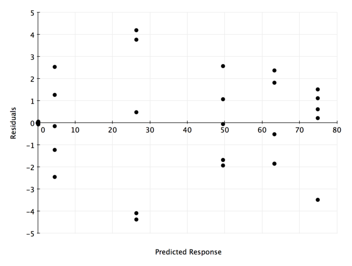
It is hard to tell whether the residuals are homoscedastic or not. Because the scale of the errors is lower than the rule of thumb necessary to feel comfortable with the results, we will say this is roughly homoscedastic. The point mass at \((0,0)\) is before any packet loss is incurred, so it natural to see the centering.
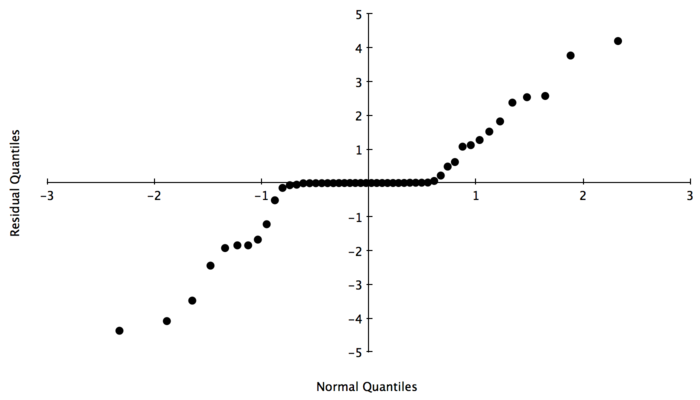
Figure 5 plots the residuals against a normal distribution. It is clear from the figure that our residuals are not normally distributed. However, the QQ-plot tells us that we have a large point mass around the origin, which is in agreement with our analysis of Figure 4. As we move away from the origin, we have the appearance of normality. We tried multiplicative models and other transformations, and the overall structure was unchanged. It is as through the residuals are actually a normal random variable and another variable that accounts for the point mass near the origin. This is intuitive: before we start incurring packet loss, our packet loss will be concentrated around zero. We will try looking at a truncated model of our results, where we only pay attention to events with a decent amount of packet loss.
In order to decide when we think our (hopefully) normally distributed residuals are kicking in, we should look at a graph of our mean loss percentage over the different number of parallel flows.
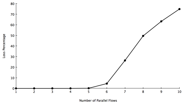
Both visually and numerically, it seems as though we only start accruing actual packet loss when we transition from 5 UDP receivers on the host machine to 6. As a result, we are going to truncate our model to only look from 6 to 10 servers. This will not change any of the numbers. We are simply trying to eliminate the large point mass at 0 loss, and only validate our model when we are actually seeing variation. Now we can plot the residuals against the predicted responses for our new model.
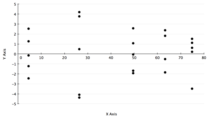
As we can see, this is almost identical to the previous graph! The only difference is it eliminates the point mass at zero, just like we wanted. We now have a stronger argument for homoscedasticity, though we are still making a judgment call based on the relatively small size of the errors.
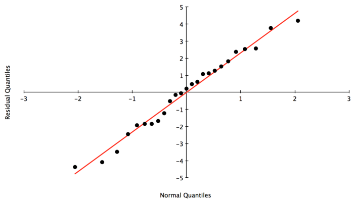
Checking the QQ-plot has the same effect. It is now fair to argue that we have normally distributed errors. The only difference between the truncated model and the original is that we have eliminated the point mass at the origin. In our opinion, this validates our entire model, and the point mass at 0 was indeed due to the nature of having zero loss.
Now that we have validated our model assumptions, we should see what claims our experiment allows us to make. We took confidence intervals of the different between two successive loss rates, i.e. it was calculated only between neighboring values of \(N\). We used a \(95%\) confidence interval. Because we took 10 observations with 5 repetitions, we use 40 degrees of freedom towards the t-value. However, because we took over 30 observations, we can instead use the z-scores of the normal distribution. Looking this up in our table gives \(z_{[0.975]} = 1.96\) [Jain91]. The calculated confidence intervals are listed in the table below:
| Effect | Confidence Interval | Significant |
|---|---|---|
| \(\alpha_2-\alpha_1\) | \((-17.66,17.66)\) | |
| \(\alpha_3-\alpha_2\) | \((-17.65,17.67)\) | |
| \(\alpha_4-\alpha_3\) | \((-17.66,17.66)\) | |
| \(\alpha_5-\alpha_4\) | \((-17.51,17.81)\) | |
| \(\alpha_6-\alpha_5\) | \((-13.27,22.05)\) | |
| \(\alpha_7-\alpha_6\) | \((4.17,39.49)\) | ✓ |
| \(\alpha_8-\alpha_7\) | \((5.52,40.84)\) | ✓ |
| \(\alpha_9-\alpha_8\) | \((-3.92,31.4)\) | |
| \(\alpha_{10}-\alpha_9\) | \((-6.07,29.25)\) |
This table statistically validates what was already intuitive from our original table of data. As we increase the number of parallel flows going into the same host machine (also increasing the number of server VMs on that host machine), we start degrading the performance. In the beginning we are still getting essentially no packet loss, so it barely changes. However, as we start hitting some resource threshold, the performance starts to worsen. We can see that the loss rate increases as we reach 6 receivers on the host machine, but it does not increase enough to be statistically significant. However, between 6 and 7 receivers on the host machine, the increase in loss is statistically significant. The same conclusion holds for the transition between 7 and 8 receivers.
We can match this against our original loss percentage data to make a decision about the number of VMs we will support on one host machine due to our UDP constraints. If we want to offer a relatively flawless experience, then capping it at 5 VMs seems the most reasonable — the loss rate should not be above 1% in my opinion. However, if we were fine with larger fluctuations in performance so long as they are not too bad, the ideal spot is at 6 VMs before we hit statistically significant degradations of performance.
Performance testing was incredibly valuable for testing our new virtual machine services in ONL. It gave us specific actions to pursue after this preliminary study, so that we can hope to maximize the performance and minimize the problems we are having. While we did have simple factorial designs, this was largely due to the guided inquiry that was done before the formal experimental design began. Had we not discarded many response variables and factors, the remaining experiment would have been huge and unwieldy. Additionally, parts of TCP do not apply to UDP and vice versa, so the narrative would have been muddled. There is much future work to be done, but this is a great starting point for provisioning virtual machine tenants in our Open Networking Laboratory. Two directions for future work include debugging the mysterious bridge packet loss problem, and analyzing the different size of UDP socket buffers (above 8KB) to reduce more socket buffer errors. The final takeaway is that, with the current hardware and software configurations, the machines that host VMs should not have more than 5 or 6 tenant VMs on them at any time, otherwise it will degrade the UDP performance to unsatisfactory levels.
I would like to thank Rahav Dor for letting me use his fantastic webpage paper template. The attention to detail is impeccable, and makes for a polished paper.