| Joe Wingbermuehle, wingbej@wustl.edu (A paper written under the guidance of Prof. Raj Jain) |
Download |
Keywords: Auto-Pipe, Laplace's Equation, Performance Analysis, Queueing Theory, Monte-Carlo Simulation, X-Language
We attempt to determine the best topology and resource mapping for an Auto-Pipe application to solve Laplace's equation. Auto-Pipe allows one to experiment with various topologies of the application and obtain timing information. We use the Monte-Carlo method for solving Laplace's equation since it represents a small, but useful application that fits nicely into the streaming framework.
Auto-Pipe is a system for creating computing pipelines across heterogeneous compute platforms [Tyson06, Franklin06, Chamberlain07]. A heterogeneous compute platform may contain a combination of CPUs, GPUs, FPGAs, or other accelerator devices. Auto-Pipe provides the user with the ability to author compute blocks to operate on a data stream. The user can then specify the topology and resource mapping of the application using Auto-Pipe's X language. This X language description is fed to the Auto-Pipe X compiler to build the application. The Auto-Pipe approach allows one to access timing information for individual blocks and to easily modify the application topology and block-to-resource mapping of the application.
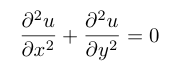
The goal of the application is to solve Laplace's equation in two dimensions (shown in figure 1.1). Laplace's equation is a second-order partial differential equation (PDE) [Strauss92]. This equation has several uses including modeling stationary diffusion (such as heat) and Brownian motion. For heat, given the temperatures at the boundaries of a two-dimensional object, solutions to Laplace's equation provide the interior temperatures after the temperatures have stabilized. The ease of solving Laplace's equation depends on the nature of the boundary conditions. An analytic solution exists for simple boundary conditions, however, for many boundaries conditions, no analytic solution exists and numerical solutions must be sought [Farlow93].
There are numerous ways to solve Laplace's equation. As previously stated, for certain simple boundary conditions a straight-forward analytical solution exists. However, it is often the case that a numerical method is required. One numerical approach is Gauss-Seidel iteration [Strauss92]. This method converges to the correct solution quickly, but it requires that the complete grid be stored in memory. Another method is Monte-Carlo simulation. This technique is provably correct [Reynolds65], but converges slowly. Nevertheless, this method is useful if only a few interior points are needed. This is because the Monte-Carlo method does not require storing the whole grid since the grid is implicit and only those points that are of interest need be computed. Further, Monte-Carlo methods work well in a pipelined framework such as Auto-Pipe [Singla08].
The Auto-Pipe application to solve Laplace's equation is made up of several compute blocks. We can replicate some blocks to achieve better performance via parallelism by dividing the work across multiple compute resources. All of the blocks considered here are implemented in C for a general purpose processor. However, Auto-Pipe would allow any of these to be re-implemented for an FPGA. Table 1.1 lists the blocks used in this application. Note that there are a few other blocks used to seed the random number generator and to read the boundary conditions, but these blocks don't contribute much to the running time so we don't consider them here.
| Block | Description |
|---|---|
| RNG | Random number generator. |
| Split | Block to distribute numbers equally among two outputs. |
| Walk | Block to perform random walks. |
| AVG | Block to take the average of two inputs. |
| Block to output the result. |
The application works by generating random numbers which are then fed to a block to perform a random walk starting from the coordinates of interest. For this application we consider all grid coordinates. The random numbers determine the direction for each stage of the random walk. The walk continues until a boundary is crossed. Once the boundary is crossed, the temperature at the boundary point is forwarded to either a print block, which saves the result to a file, or an average block, which averages the results of two inputs. The application continues this process many times for each coordinate in a rectangular region. Note that in a real use of this application one would probably only be interested in few locations, but for the purpose of performance analysis, we consider the whole grid.
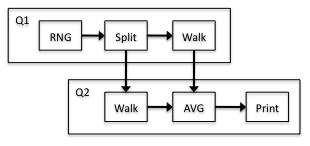
There are multiple ways to divide the random walks among compute resources. One method is to configure the block used to generate random numbers to feed a block that splits the output among multiple walk blocks. A second method is to replicate the random number generation blocks along with the walk blocks by using different random number seeds for each random number generation block. In either case, we feed the results from the random walk blocks to a block that averages them before we send the averages to a print block to be recorded. Given a single compute node, the topology of this application is straight-forward. However, even with only two processors, there are several possible block topologies and several resource mappings that may make sense. Our goal is to determine the best topology and resource mapping.
As stated above, our goal is to determine the best block topology and resource mapping. To do this, we must first define what it means to be the the best. Next, we determine what is to be measured and isolate the parameters that may affect that measurement. Finally, we select a method for evaluating the performance.
The first step in determining the best mapping is to define the metrics of interest. We assume no application errors and that the service is always performed correctly. Given this, the performance metrics are response time, throughput, and resource utilization [Jain91]. For this application, we will focus on throughput. Throughput is defined by the number of jobs that can be completed per unit time. Here we define a job as a point whose temperature is to be evaluated.
System parameters affecting performance include:
Workload parameters include:
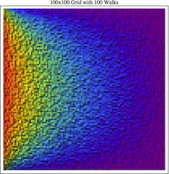
The grid size was fixed to 100x100 and the boundary conditions were set to a square containing the grid. The temperature at the boundary was set to 0 for three sides and 100 for the fourth side. One hundred random walks were done at each grid coordinate. The output of the application gives a 100x100 grid of temperatures. A plot of the output using colors to represent temperatures (blue being 0 and red being 100) yields an image as seen in figure 2.1.
For all timings performed, the system parameters will remain fixed. The system used is a dual dual-core 2.2 GHz AMD Opteron system with 1 MB L2 cache and 8 GB of system memory. The grid size, boundary conditions, and number of random walks will also remain fixed. The grid size is fixed to 100x100. The boundary is fixed as the whole grid area with three corners set to 0 and the fourth set to 100. The number of random walks is set to 100 for each coordinate. Only the application topology and resource mapping will be varied.
To determine the best resource mapping and application topology, we will explore several possibilities. Since the topologies and resource mappings for differing numbers of compute resources vary, we will treat this as a single factor experiment for each set of compute resources. We refer to this factor as a "mapping". To uniquely identify a mapping, we prepend the number of processors to the name of the mapping. For example, mapping 4A is a mapping on to four processors.
In order to explore possible topology and resource mappings for the application, we use an analytic model. We use results from queueing theory to model several possible topologies and resource mappings. [Dor10a] and [Dor10b] have shown queueing theory to be a useful modeling tool for streaming applications.
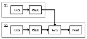
To model this application as an open queueing network, we define each processor as being an M/M/1 queue. This allows us to use operational laws to reason about the network. If we can determine the demand for each processor, the operational laws will allow us to determine other useful properties of the network, such as processor utilization and throughput. Demand is defined by the service time multiplied by the number of visits. Since it is often the case that several stages of the pipeline get assigned to the same processor, we compute the demand for each processor by summing the demand for each block mapped to that processor scaled by the size of the problem at that point. To get the demands for each block, we obtain timings for the simple topology shown in figure 3.1.
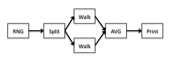
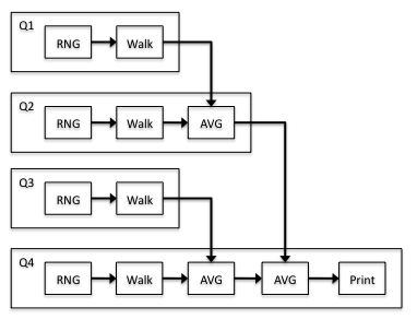
The resource mapping does not matter for determining the demand since we only care about the individual block timings. This is because the amount of processor time spent executing each block is the same if the block is run in parallel with other blocks or serially. Also note that because the walk block is replicated in simple topology, we use the sum of the demands for the total walk demand. Given the per-block demand for the simple topology, one can use operational laws to determine the bottleneck and demand for more complex topologies and resource mappings. Consider the four-queue system in figure 3.2.
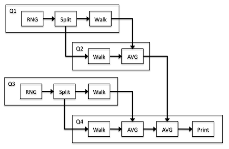
In this example, there are four queues (processors), each of which has multiple blocks assigned to it. Half of the RNG and Split jobs from the simple topology and a quarter of the Walk jobs will get processed on the first processor. We apply similar reasoning to the other processors to obtain the following results for the demand of each processor:
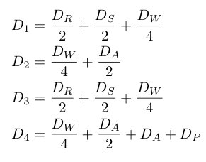
Now we can compute the bottleneck, which is the processor with the highest demand. Given the bottleneck processor, we can compute the maximum throughput using the following equation:
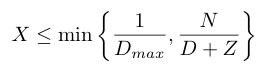
Here N is the number of jobs, Dmax is the demand of the bottleneck processor, D is the total demand of the system, and Z is the think time, which is zero for this system. Since N is large in this application, the throughput will be the inverse of the bottleneck processor. To get the execution time we can multiply the demand by the number of jobs. The processor utilization is also easy to compute by multiplying the processor demand by the throughput of the complete system. This gives a simple way to estimate the throughput, execution time and processor utilization for an arbitrary topology and resource mapping based only on the timings of the individual blocks.
To use our model, we must have the demand for the various blocks for the topology in figure 3.1. We can use the total running time of each block and divide by the number of jobs to determine the demand for each block. Note that there are 10000 jobs (width * height). We obtained the timings directly from Auto-Pipe, which provides a summary of the execution times for each block in the system. Auto-Pipe also provides a means to obtain traces [Gayen07], but this level of detail is not needed here.
Using Auto-Pipe, the simple topology in figure 3.1 was run on a single processor five times and the average block time was recorded. Table 3.1 shows the results. We compute the demand for each block by dividing the time by the number of jobs.
| Block | Run Time (seconds) | Standard Deviation | 90% Confidence Interval |
|---|---|---|---|
| RNG | 3.92004126 | 0.150262 | (3.77677, 4.06331) |
| Split | 0.14195219 | 0.00487290 | (0.137306, 0.146598) |
| Walk | 25.2997121 | 0.00738346 | (25.2927, 25.3068) |
| AVG | 0.0007355 | 1.54890E-5 | (0.000707320, 0.000750268) |
| 0.004684558 | 3.29668E-5 | (0.00465313, 0.00471599) |
The fact that the confidence intervals do not overlap indicates that all of the block timings are distinct with a 90% confidence. This means that it is not possible to directly substitute one block for another.
We analyze several mappings. These mappings are not exhaustive and may not be optimal, but they represent what we consider to be reasonable selections for dividing the work evenly. First we consider two-processor mappings and then four-processor mappings.
Figure 3.3 shows the first two-processor mapping (mapping 2A):
From the model, we see that the demand for processor 1 is 0.00146099 and the demand for processor 2 is 0.00146153. Thus, processor 2 is the bottleneck and the throughput is 684.215 jobs/second. Processor 1 has a 99.9629% utilization and processor 2 has a 100.0000% utilization. Combining the throughput with the number of jobs gives us 14.6153 seconds for the execution time. Figure 3.4 shows the second two-processor mapping (2B):
From the model, we can determine the demand of processor 1 to be 0.00167118 and the demand of processor 2 to be 0.00126553. Thus, processor 1 is the bottleneck. The throughput is 598.378 jobs/second with processor 1 at 100.000% utilization and processor 2 at 75.7264% utilization. The execution time is 16.7118 seconds. Therefore, the model predicts that mapping 2A is better.
Now we consider four-processor mappings. Figure 3.2 (above) shows the first four-processor mapping (4A). The model predicts the throughput of mapping 4A to be 1196.76 jobs/second and the running time to be 8.35592 seconds. Figure 3.5 shows a second four-processor mapping (4B):
The model predicts the expected throughput of mapping 4B to be 1367.85 jobs/second and the running time to be 7.31073 seconds. Thus, we expect mapping 4B to be better than mapping 4A. Finally, figure 3.6 shows a third four-processor mapping (4C):
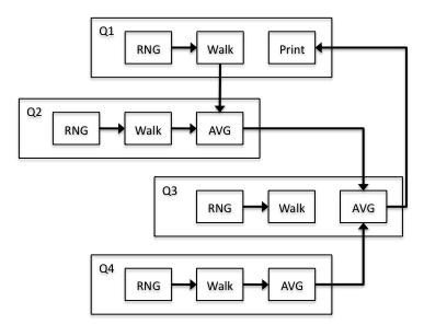
Using the model again, we predict the expected throughput of mapping 4C to be 1369.40 jobs/second and the running time to be 7.30247 seconds. This gives mapping 4C a slight edge over mapping 4B. Table 3.2 shows a summary of the model predictions:
| Mapping | Run Time (seconds) | Throughput (jobs/second) |
|---|---|---|
| 2A | 14.6153 | 684.215 |
| 2B | 16.7118 | 598.378 |
| 4A | 8.35592 | 1196.76 |
| 4B | 7.31073 | 1367.85 |
| 4C | 7.30567 | 1369.40 |
To verify the analytic model, we measured the execution times of the mappings above. We then converted the execution times to throughputs by dividing the number of jobs by the execution time. Finally, we tested these results for statistical significance and compared with the results predicted using the analytic model.
Using Auto-Pipe, we compiled the mappings presented in section 3.3 and ran each five times. As previously described, we used the average execution time to compute the throughput. Table 4.1 shows the results:
| Mapping | Run Time (seconds) | Throughput (jobs/second) |
|---|---|---|
| 2A | 14.5703 | 686.327 |
| 2B | 17.4584 | 572.791 |
| 4A | 8.62328 | 1159.65 |
| 4B | 7.31052 | 1367.89 |
| 4C | 7.30247 | 1369.40 |
An analysis of variance (ANOVA) for the two-processor mappings reveals that the mapping accounts for 99.8452% of the variation and errors account for 0.154784% of the variation. For the four-processor mappings, the mapping accounts for 99.8101% of the variation and and errors account for 0.189821% of the variation. An F-Test shows that the mapping is significant at a 90% confidence level for both the two- and four-processor mappings.
We compute r2 to determine if the predictions from the queueing model and the measurements are significantly different. The result is r2 = 0.999935. Thus, not only does the model accurately predict which mapping is better, it also does a good job at estimating the throughput. Despite this, it should be noted that the model has limitations and we have only shown the model to be good for certain parameters.
The results above allow us to evaluate the best resource mapping of those considered for both the 2-processor and 4-processor cases. Both the model and the measurements agree that mapping 2A is the best 2-processor mapping and mapping 4C is the best 4-processor mapping. We emphasize that not all possible mappings are considered and if additional resources are utilized, additional work would be needed to ascertain the best mapping. Nevertheless, the model allows us to evaluate the performance of a topology and resource mapping without actually running the application. The experimental results suggest that the queueing model works well for this problem.
As previously stated, the model is good for the problem as shown here, however, it has several limitations. First, the model does not take communication delays or other overhead into account. Further, the model was only used for a single problem size. It is unknown if the model would correctly rate topologies for a different problem size.
Our goal was to determine the best resource mapping and block topology for an application to solve Laplace's equation. To do this, we defined a way to rank the topologies and devised a simple model based on queueing theory. We used timing information gathered from Auto-Pipe to seed the model. Next, we compared various topologies to determine the best two-processor and four-processor topology. Finally, we compared the predicted responses with empirical results to validate the model.
Future work could be done to expand the model to take the problem size and communication costs into account. Also not considered here is whether the model would work for comparing blocks implemented on different types of computing resources, such as FPGAs or GPUs.
In order of importance:
[Tyson06]
E. J. Tyson, "Auto-Pipe and the X Language: A Toolset and Language
for the Simulation, Analysis, and Synthesis of Heterogeneous
Pipelined Architectures," Master's Thesis, Washington University
Dept. of Computer Science and Engineering, August 2006.
The original thesis on which the Auto-Pipe system is based.
http://sbs.wustl.edu/pubs/thesis_ejt.pdf
[Chamberlain07]
R. D. Chamberlain, E. J. Tyson, S. Gayen, M. A. Franklin, J. Buhler,
P. Crowley, and J. Buckley.
"Application Development on Hybrid Systems,"
In Proc. of Supercomputing (SC07), pages 1-10, November 2007.
Paper on using Auto-Pipe for application development and performance
modeling.
http://sc07.supercomputing.org/schedule/pdf/pap442.pdf
[Franklin06]
M. A. Franklin, E. J. Tyson, J. Buckley, P. Crowley,
and J. Maschmeyer.
"Auto-Pipe and the X Language: A Pipeline Design Tool and
Description Language"
In Proc. of Int'l. Parallel and Distributed Processing Symposium,
pages, 10 pages, April 2006.
Paper on using Auto-Pipe to develop applications.
http://www.arl.wustl.edu/~pcrowley/ftbcm06.pdf
[Dor10a]
R. Dor, “Against all probabilities: A modeling paradigm for streaming
applications that goes against common notions,” Dept. of Computer
Science and Engineering, Washington University in St. Louis,
Tech. Rep. WUCSE-2010-30, 2010.
Thesis on modeling streaming applications using queueing theory.
http://cse.wustl.edu/Research/Lists/Technical%20Reports/Attachments/924/RahavDor_thesis.pdf
[Dor10b]
Rahav Dor, Joseph M. Lancaster, Mark A. Franklin, Jeremy Buhler,
and Roger D. Chamberlain, "Using Queuing Theory to Model Streaming
Applications,"
In Proc. of 2010 Symposium on Application Accelerators in High
Performance Computing (SAAHPC), 3 pages, July 2010.
Paper describing how M/M/1 queues are applied to streaming
applications.
http://www.cse.wustl.edu/~roger/papers/dlfbc10.pdf
[Singla08]
Naveen Singla, Michael Hall, Berkley Shands,
and Roger D. Chamberlain, "Financial Monte Carlo Simulation on
Architecturally Diverse Systems," in Proc. of Workshop on
High Performance Computational Finance, pages 1-7,
November 2008.
Paper detailing how a financial Monte-Carlo simulation
is performed using heterogeneous compute resources in the Auto-Pipe
environment.
http://www.cse.wustl.edu/~roger/papers/shsc08.pdf
[Jain91]
Raj Jain, "The Art of Computer Systems Performance Analysis:
Techniques for Experimental Design, Measurement, Simulation,
and Modeling," Wiley, April 1991, ISBN: 0471503363.
Book containing information on experimental design and queueing theory.
[Reynolds65]
J. F. Reynolds, "A Proof of the Random-Walk Method for Solving
Laplace's Equation in 2-D," The Mathematical Gazette,
49(370), pages 416-420, December 1965.
Paper that provides a proof of the Monte-Carlo method for solving
Laplace's equation.
http://www.jstor.org/pss/3612176
[Strauss92]
W. A. Strauss, "Partial Differential Equations: An Introduction,"
Wiley, 1992, ISBN: 0471548685.
Book on partial differential equations providing information on
solving Laplace's equation.
[Farlow93]
S. J. Farlow, "Partial Differential Equations for Scientists and
Engineers," Dover Publications, September 1993,
ISBN: 048667620X.
Book on partial differential equations providing additional
details on when Laplace's equation has an analytic solution.
[Gayen07]
S. Gayen, E. J. Tyson, M. A. Franklin, and R. D. Chamberlain.
"A Federated Simulation Environment for Hybrid Systems"
In Proc. of 21st Int'l Workshop on Principles of Advanced and
Distributed Simulation, pages 198-207, June 2007.
Paper describing X-Sim, which is a simulation environment
for the Auto-Pipe environment.
http://portal.acm.org/citation.cfm?id=1249025
| ANOVA | Analysis of Variance |
| CPU | Central Processing Unit |
| FPGA | Field-Programmable Gate Array |
| GPU | Graphics Processing Unit |
| PDE | Partial Differential Equation |
| RNG | Random Number Generator |