Comparison of Real-time Scan Conversion Methods With an OpenGL Assisted Method
Abstract:
Ultrasonic scan conversion, which is needed to transform polar coordinate ultrasound data into Cartesian coordinate data consumable by standard graphics systems, is one of the performance bottlenecks of an ultrasound system. Many current systems employ custom hardware or DSPs to create scan converters. However with the increasing speed of computers and their graphics systems, PCs are now a viable platform for ultrasound systems. This paper proposes using the texture mapping capabilities of OpenGL and leverage the graphics system to perform scan conversion.
The new OpenGL algorithm effectively off-loads the heavy lifting of scan conversion, the thousands of interpolations that must be performed, to the GPU. This should dramatically improve the throughput of the conversion and free up CPU cycles on the general purpose processor for other tasks. This paper compares the new OpenGL algorithm to three traditional methods: nearest neighbor, linear interpolation, and bilinear interpolation, and compares their throughput and noise performance in order to demonstrate the viability of using OpenGL to perform scan conversion.
Keywords:
ultrasound, scan conversion, OpenGL, interpolation
Table of Contents
- Introduction
- Background Information
- Ultrasound System Architecture
- B-mode Image Frames
- Basic Scan Conversion
- Traditional Scan Conversion Methods
- Nearest Neighbor
- Linear Interpolation
- Bilinear Interpolation
- Optimal Approximation
- OpenGL Assisted Conversion
- Experimental Methods and Results
- Throughput Experiments
- Throughput Results
- Error Estimation Experiments
- Error Estimation Results
- Conclusions
- References
- Appendix A - Abbreviations
1. Introduction
Ultrasound is the most popular and inexpensive non-invasive medical imaging technologies. With the introduction of portable and handheld ultrasound systems, ultrasound is being used not only in hospitals, but in clinics, private practices, and maybe someday in our households. This ever-increasing use of ultrasound drives the need to develop faster, smaller, and more efficient ways to collect ultrasound data and convert it into usable and viewable images. One of the key processes in generating viewable ultrasound images that may be improved is scan conversion.
In the past, ultrasonic scan converters have been implemented using custom hardware, digital signal processors (DSP), and field programmable gate arrays (FPGA) [Richard94, Zar93, Kassem05, Chang08]. However with the advancement of general-purpose processors and graphics processors, it is becoming more common to push much, if not all, of the image processing in to software. The aim of this paper is to compare the speed and effectiveness of some common scan conversion algorithms implemented in software along with a new algorithm that utilizes the standard OpenGL libraries which in turn leverage the system's graphics hardware.
2. Background Information
2.1 Ultrasound System Archtecture
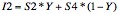
The block diagram in Fig. 1 illustrates a simple model of an ultrasound probe with a single element transducer. The front-end uses a high frequency, high voltage pulse to excite the transducer to produce ultrasound waves. The sound waves, or echoes, that bounce back from the tissue excite the transducer to produce an electric signal. The signal is amplified by the front-end and processed to make the data more suitable for human visual consumption. The echo signals are then digitized, scan converted, and transmitted to the graphics subsystem for display.
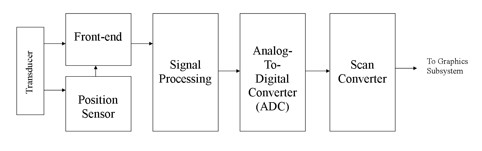
Fig. 1 Block diagram of a simple ultrasound system
2.2 B-mode Image Frames
Each echo signal, or A-mode vector, that is digitized and stored represents the echo pattern from the tissue that the transducer is aimed at. In the case of a mechanical sector scan probe, a motor moves the transducer along a curved path in order to interrogate different areas of the tissue. The probe tracks the position of the transducer and directs the front-end to pulse the transducer and receive A-mode vectors at fixed, angular intervals. Once the probe has collected vectors from all of the specified angles, a B-mode frame is formed. The B-mode frame is simply the two dimensional (2D) array of formed by storing all the A-mode vectors, from all of the angles, in consecutive order. The B-mode frame is then sent to the scan converter, so that an image can be formed.
While many new ultrasound system use transducer arrays, which do not require motors, the concept of B-mode frames is still the same. Specialized front-ends and beam-formers are used to aim the ultrasound beam at a specific region of tissue to form an A-mode vector. The vectors are then stored as B-mode frames and scan converted in the same manner as image formed by a mechanical scanning probe.
2.3 Basic Scan Conversion
The need for scan conversion is driven by the way that the B-mode frames are formed. Since an angular distance separates each vector and the sampling rate of each vector is fixed, then the B-mode frame is stored in polar coordinate form [Schueler84]. Thus scan conversion is needed to transform the polar coordinate data into standard Cartesian coordinates that are needed by standard graphics subsystems [Ophir79]. Figures 2 and 3 illustrate a B-mode frame of a human prostate before and after scan conversion.
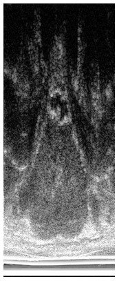
Fig. 2 Raw B-mode image data
(before scan conversion) |
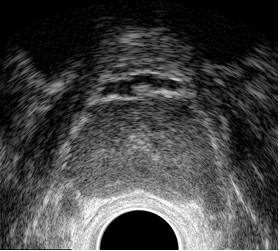
Fig. 3 B-mode image after scan conversion |
Given that the sampling rate is fixed and the there is no over sampling, then there is no one-to-one mapping between the raw B-mode frame and the output image. Thus some form of interpolation is typically performed during the scan conversion process. This paper will compare the performance of the interpolation as well as the throughput of three widely used scan conversion algorithms (nearest neighbor, linear interpolation, and bilinear interpolation) with a new OpenGL assisted scan conversion algorithm.
3. Traditional Scan Conversion Methods
3.1 Nearest Neighbor
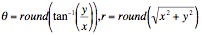
The first and simplest method for scan conversion is nearest neighbor. In this method the closest data point to the needed pixel is used, and no interpolation is performed. Thus a pixel at location (x,y) will have a value equal to that of the data point located at θ, r in the raw B-mode frame.
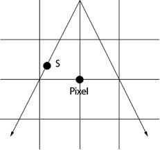
Fig. 4 Nearest Neighbor algorithm. The value of the closest sample (S) become the value of the pixel
 | [1] |
3.2 Linear Interpolation
The next method uses over-sampled vectors coupled with simple linear interpolation to perform the conversion. As shown in Fig. 5, the data is over-sampled in the radial direction providing two data points on adjacent vectors that lie approximately along a linear path with the needed pixel. Simple linear interpolation can be performed between these two data points in order to determine the value of the pixel [Richard94]. Equation [2] shows how the interpolation is computed; A is the value of data point A along vector θ1, B is the value of data point B along vector θ2, and C is the distance between the pixel and B.
Fig. 5 Linear Interpolation algorithm. Given 4x over-sampling in the radial direction, the pixel is computed using the two closest pixels from adjacent vectors. Figure borrowed from [Richard94].
 | [2] |
3.3 Bilinear Interpolation
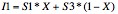
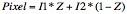
Bilinear interpolation is performed using four data points from adjacent vectors to compute the value for the needed pixel. This method does not require over-sampled vectors, but it does require more computation than the previous linear interpolation method. Fig. 6 shows the relationship between the four data points and the pixel. In order to obtain the pixel value, three linear interpolations must be performed. Two data points are interpolated between S1 and S3 and between S2 and S4. Then the pixel value is calculated by interpolating between the two new data points. These three interpolations are described by equations [Kassem05, Chang08].
Fig. 6 Bilinear Interpolation algorithm. The closest four points on the two adjacent vectors are used to calculate the value of the pixel. Figure borrowed from [Richard94].
In equation [3], X is the distance between I1 and S3, in equation [4], Y is the distance between I2 and S4, and in equation [5], Z is the distance between the pixel and I2. Combining these three equations gives equation [6], where A, B, C, and D represent the simplified constants obtained after combining these equations.
 | [6] |
3.4 Optimal Interpolation
Optimal approximation is not typically used for real-time scan conversion because of the large amount of computation that is required, but it is a useful tool for creating near optimal images that can be used to estimate the error of the previously described methods. This method involves up-sampling the raw B-mode frame in both the radial and the azimuth directions using the sin(x)/x interpolator [Richard94, Stark81]. The interpolation is accomplished with the following procedure: perform the FFT in both directions on the raw frame data, pad the transformed data, and perform the inverse FFT; this method is further described in [Richard94]. Once the data has been interpolated in both directions, the optimal scan converted image is created using the nearest neighbor method on the interpolated raw data.
4. OpenGL Assisted Conversion
The new OpenGL assisted scan conversion algorithm harnesses the power of the standard OpenGL library and, in turn, the graphics hardware present on the PC. The algorithm uses the texture mapping function of OpenGL to map the raw B-mode data onto a sector shape that fits the dimensions of the scan converted image [Woo91]. The sector is defined using adjacent quadrilaterals (quads) as shown in Fig. 7. Two of the vertices of each quad are always at the origin (also the axis of rotation in the mechanical system) and the other two vertices lie on the outside of the sector at distance r from the origin. Since two of the vertices of each quad are the same point, the sector could be defined using triangles, however the texture mapping would not be applied correctly and the image would be skewed [Segal06].
Fig.7 Quadrilateral vertices mapped to texture coordinates. Each vertex on the left (V1-V4) is mapped to texture coordinate (T1-T4) that corresponds to the correct angle and radius.
As the quads are defined, texture coordinates are mapped to each vertex. Each texture coordinate refers to a specific location in the raw B-mode data, and once a texture coordinate has been assigned to all four vertices of a quad the OpenGL library can map that portion of the data onto the sector. The code excerpt in Fig. 8 demonstrates how the quads and texture coordinates are defined. Each time through the loop two vertices are defined at the specified angle, one at the origin and one on the edge of the sector. The texture coordinates mapped to these vertices correspond to the beginning point and ending point of the one of the vectors in the B-mode image.
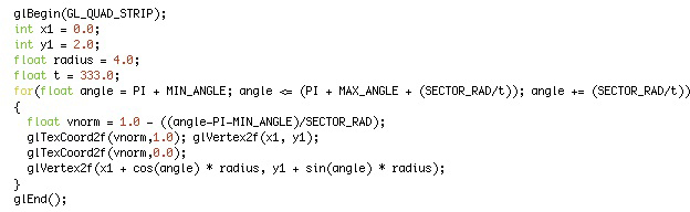
Fig. 8 Code example illustrating sector definition and texture coordinate mapping. x1,y1 is the origin, t is the number of quads used to define the sector. The sector start at angle PI + MIN_ANGLE and goes to PI + MAX_ANGLE since the sector must be facing downward.
Once the entire mapping is complete, the OpenGL library performs all of the necessary interpolations to define each pixel in the final image. OpenGL can be directed to handle the interpolations in two basic ways: nearest and linear. Using the nearest option, the library finds the data point in the texture (the B-mode data) and uses is value for the value of the pixel, just like the nearest neighbor algorithm described in 3.1. Similarly the linear option directs the library to perform bilinear interpolation using the four closest data points in the texture. In this implementation the linear option (bilinear interpolation) is used [OpenGL].
While the interpolation routines are the same as the traditional scan conversion methods, the underlying implementation differs greatly. Since the interpolation occurs within the OpenGL library this new algorithm can leverage the processing power of the graphics hardware of the PC. Furthermore, OpenGL is platform independent and can interact with the graphics hardware of any standard PC. These advantages should provide better throughput for the ultrasound system while not adding significant noise to the image.
5. Experimental Methods and Results
5.1 Throughput Experiments
The first set of experiments is designed to investigate the throughput of the scan conversion process. Two factors were manipulated during the course of the experiment: the algorithm and the size of the output image. Both of these factors control how many interpolations must be computed to form the output image, and they should be the most significant factors affecting the performance of the conversion process. In this experiment, the content of the image is not used as a factor since the content does not affect the number or execution time of the interpolations. A full factorial design with replications was chosen as the experimental model [Jain91]. In this design each of the four algorithms are run with three different output image sizes and each experiment is replicated five times to give a total of 60 experiments.
Given the relative simplicity of each of the algorithms, direct measurement of the throughput was chosen rather than an analytical approach. Each of the algorithms is coded in C, and each experiment was run on a MacBook Pro with OS 10.4 and an ATI Radeon X1600 graphics chipset with 128 MB of video RAM. To ensure that the algorithms using the general purpose CPU obtained maximum throughput, the nearest neighbor, linear interpolation, and bilinear interpolation algorithms are coded such that they used both processor cores in a shared memory approach. The workload is divided between the cores using a standard row decomposition method on the output image data. To measure the throughput a sample image was scan converted 500 times, the time was recorded, and the throughput (frames/s) was computed.
5.2 Throughput Results
Table 1 Throughput Results (frames/sec)
| Size |
Algortithm |
| | NN | LI | BIL | GL |
| 668x597 | 251.76 | 178.57 | 73.52 | 284.58 |
| | 254.19 | 184.16 | 74.52 | 281.06 |
| | 254.45 | 181.23 | 74.69 | 284.74 |
| | 253.42 | 181.95 | 74.31 | 284.25 |
| | 253.42 | 175.13 | 74.57 | 283.93 |
| 501x448 | 371.47 | 261.64 | 122.31 | 375.38 |
| | 358.42 | 274.88 | 124.75 | 373.69 |
| | 358.68 | 273.82 | 124.25 | 371.75 |
| | 362.06 | 276.40 | 123.73 | 376.22 |
| | 367.65 | 274.73 | 125.09 | 377.36 |
| 334x299 | 520.83 | 437.06 | 242.01 | 909.09 |
| | 521.38 | 428.81 | 239.69 | 891.27 |
| | 519.21 | 429.55 | 240.62 | 884.96 |
| | 505.05 | 440.92 | 239.46 | 891.27 |
| | 517.60 | 440.14 | 240.04 | 891.27 |
NN = Nearest Neighbor, LI = Linear Interpolation,
BIL = Bilinear Interpolation, GL = OpenGL Assisted
Table 2 Throughput ANOVA Table
| Component | Sum of Squares | % Variation | Degrees of Freedom | Mean Square | F Computed | F-Table |
| SSY | 9290311 | | 60 | | | |
| SS0 | 6708706 | | 1 | | | |
| SST | 2581604 | 100 | 59 | | | |
| SSA (Algorithm) | 1084022 | 41.99 | 3 | 361341 | 17107 | 2.23 |
| SSB (Size) | 1124118 | 43.54 | 2 | 562059 | 26610 | 2.44 |
| SSAB | 372451 | 14.43 | 6 | 62075 | 2939 | 1.92 |
| SSE | 1014 | 0.04 | 48 | 21.12 | | |
Table 1 shows the results of all 60 of the throughput experiments that were run. Using standard analysis of variance techniques, both the size of the image and the algorithm were found to be statistically significant factors with 90% confidence [Jain91]. As shown in the ANOVA table (Table 2), the algorithm and the image size explain 42% and 44% of the variation in throughput respectively. Furthermore the OpenGL algorithm is, on average, much faster than the three traditional algorithms as shown in Table 3.
Table 3 Traditional Conversion Throughput vs. OpenGL Throughput
| Algorithm | Mean Throughput (fps) | Difference (OpenGL - x) (fps) | Error |
| NN | 377.97 | 139.42 | +/- 3.3 |
| LI | 295.93 | 221.46 | +/- 3.3 |
| BIL | 146.24 | 371.15 | +/- 3.3 |
| OpenGL | 517.39 | 0 | +/- 3.3 |
5.3 Error Estimation Experiments
The second set of experiments is designed to investigate the error of the scan conversion methods as compared to the optimal approximation. Again two factors are controlled during the experiment: algorithm and image content. Since noise, when compared to optimal, should not be affected by the size of the image, it is not considered in this experiment. The algorithms will be the same as the previous throughput experiment and use the same implementation. Since the content of the image can affect the level of noise, six different images are compared: heart, kidney, liver, and three different phantoms. A full factorial design was also chosen for this set of experiments, however no replications are used [Jain91]. In this design each of the four algorithms is run on each of the six images yielding 24 experiments.
The original image data from the previous paper [Richard94] was obtained from the authors and as well as the S/N Power data for the nearest neighbor, linear interpolation, and the bilinear interpolation algorithms. Using the same methods, the original B-mode data is scan converted using the OpenGL assisted method and is compiled with the data from the other algorithms to produce the final data shown in Table 4. The signal power is estimated by the sum of the squares of the optimal image pixels and the error power is estimated by the sum of the squares of the difference image.
5.4 Error Estimation Results
Table 4 Error Estimation Results (S/N Power dB)
| Image | Algorithm |
| | NN | LIN | BIL | GL |
| heart | 21.7 | 26.0 | 23.4 | 26.4 |
| kidney | 20.3 | 24.8 | 22.0 | 24.6 |
| liver | 20.6 | 24.8 | 22.3 | 23.8 |
| phantom 1 | 21.5 | 26.5 | 23.1 | 24.4 |
| phantom 2 | 21.6 | 25.6 | 23.3 | 24.5 |
| phantom 3 | 24.1 | 30.0 | 25.7 | 23.1 |
NN = Nearest Neighbor, LI = Linear Interpolation,
BIL = Bilinear Interpolation, GL = OpenGL Assisted
Table 5 Error Estimation ANOVA Table
| Component | Sum of Squares | % Variation | Degrees of Freedom | Mean Square | F Computed | F-Table |
| SSY | 13844 | | 24 | | | |
| SS0 | 13733 | | 1 | | | |
| SST | 11.3 | 100 | 23 | | | |
| SSA (Algorithm) | 68.98 | 61.97 | 3 | 22.99 | 17.23 | 2.49 |
| SSB (Size) | 22.31 | 20.04 | 5 | 4.46 | 3.34 | 2.27 |
| SSE | 20.02 | 17.97 | 15 | 1.33 | | |
Table 4 shows the results of all 24 of the error experiments that were run. Again using standard analysis of variance techniques, both the size of the image and the algorithm were found to be statistically significant factors with 90% confidence [Jain91]. As shown in the ANOVA table (Table 5), the algorithm and the image size explain 62% and 20% of the variation in S/N power respectively. However, as seen in Table 6, the OpenGL algorithm is not statistically different from the nearest neighbor or the bilinear interpolation algorithms. Since the OpenGL algorithm uses bilinear interpolation to determine the pixel values in the output image the noise performance should be close to that of the traditional bilinear algorithm. It should also be noted that the linear interpolation algorithm gains much of its added S/N power through the use of over-sampled vectors, and the OpenGL algorithm should also benefit from having more sample data possibly giving it a better S/N power.
Table 6 Traditional Conversion Throughput vs. OpenGL Throughput
| Algorithm | Mean S/N Power (dB) | Difference (OpenGL - x) (dB) | Error |
| NN | 21.63 | 2.83 | +/- 1.42 |
| LI | 26.28 | -1.82 | +/- 1.42 |
| BIL | 23.30 | 1.17 | +/- 1.42 |
| OpenGL | 24.47 | 0 | +/- 1.42 |
6. Conclusions
In terms of throughput the new OpenGL algorithm is much faster than the traditional linear interpolation and bilinear interpolation algorithms. By leveraging the power of the graphics system of the PC the OpenGL algorithm is not only able to provide more throughput, it off-loads some of the work from the general purpose CPU. With the performance bottleneck of scan conversion pushed onto the GPU, the CPU is now free to perform other operations necessary for the ultrasound system such as signal processing, handling user input, or data management.
Furthermore, the OpenGL algorithm does not sacrifice noise performance for the speed gains. It has approximately the same noise performance of the traditional bilinear interpolation algorithm, which makes it as good as many current ultrasound systems.
Using OpenGL is not only a relatively easy way to implement an ultrasonic scan converter, it is a much more efficient use of a systems resources. It can provide higher throughput than traditional methods without adding significant noise to the images. The algorithm also makes use of standard software libraries (OpenGL) as well as off-the-shelf hardware, which may eliminate the need for the custom hardware and DSPs used to implement high frame rate scan converters. This in turn can lower the cost and development time of new ultrasound systems without sacrificing noise performance for speed.
References
[Richard94] Richard WD, Arthur RM. Real-time ultrasonic scan conversion via linear interpolation of oversampled vectors. Ultrason Imaging. 16, 109-23 (1994).
[Zar93] Zar DM and Richard WD, A scan engine for standard B-mode ultrasonic imaging,
Annual ASEE Conf. (1993).
[Kassem05] Kassem A, Sawan M, Boukadoum M, A new digital scan conversion architecture for ultrasonic imaging system. Journal of Circuits, Systems & Computers; Apr 2005, Vol. 14 Issue 2, p367-382, 16p.
[Chang08] Chang JH, Yen JT, Shung KK. High-speed digital scan converter for high-frequency ultrasound sector scanners. Ultrasonics, 48(5), 444-52 (2008).
[Schueler84] Schueler HL, Lee H, and Wade G., Fundamentals of digital ultrasonic imaging,
IEEE Trans. Sonics Ultrasonics SU-31,195-217 (1984).
[Ophir79] Ophir J, and Maklad NF, Digital scan converters in diagnostic ultrasound imaging, Proc. IEEE 67, 654-664 (1979).
[Stark81] Stark H, Woods J, Paul I, and Hingorani R, An investigation of computerized tomography by direct fourier inversion and optimum interpolation, IEEE Trans. Biomed. Engr. BME-28, 296-505 (1981).
[Woo91] Woo M, Neider J, Davis T, and Shreiner D, OpenGL Programming Guide, Silicon Graphics, 1991.
[Segal06] Segal M and Akeley K, The OpenGL Graphics System: A Specification, Version 2.1, Silicon Graphics, 2006.
[OpenGL] OpenGL 2.1 Reference Pages, http://www.opengl.org/sdk/docs/man/, Manual Pages for all OpenGL 2.1 functions.
[Jain91] Jain, R, The Art of Computer Systems Performance Analysis, John Wiley & Sons, 1991.
Appendix A - Abbreviations
CPU - Central Processing Unit
GPU - Graphics Processing Unit
OpenGL - Open Graphics Library
DSP - Digital Signal Processor
FPGA - Field Programmable Gate Array
Last modified on November 24, 2008
This and other papers on latest advances in performance analysis are available on line at http://www.cse.wustl.edu/~jain/cse567-08/index.html
Back to Raj Jain's Home Page