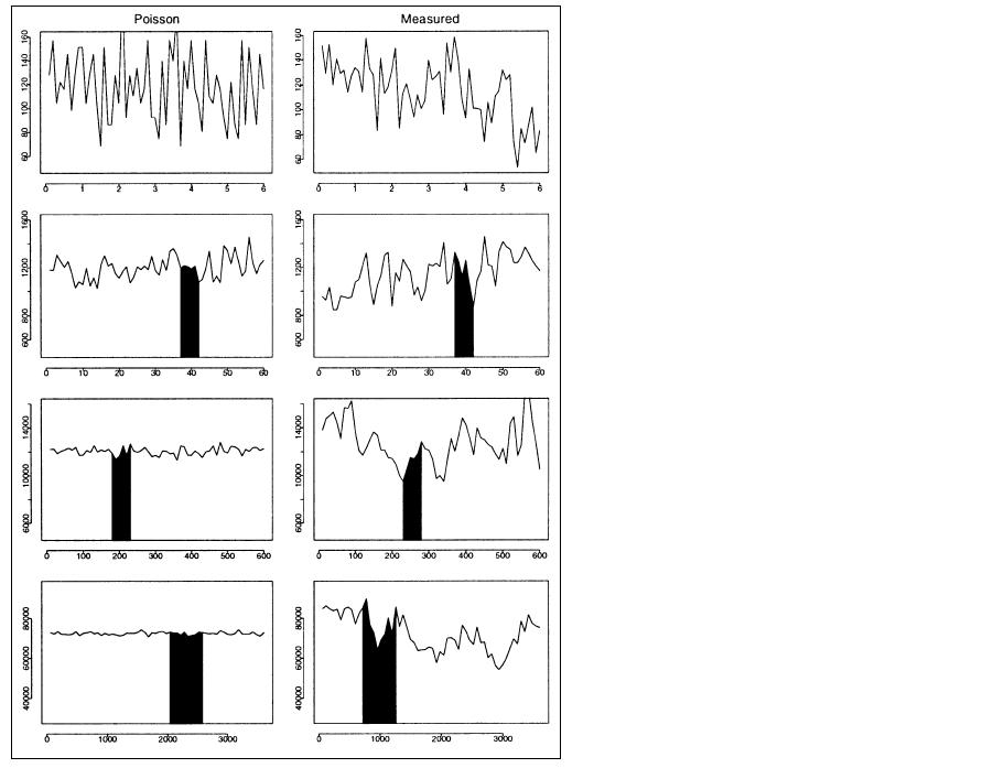
Figure 1: Synthetized traffic from a Poisson model vs. Internet traffic to which its mean and variance were fit, viewed over three orders of magnitude.
(from [willinger98where])
The first traffic model, based on Poisson processes, was born in the context of telephony, where call arrivals could be considered independent and identically distributed and "holding times" followed an exponential distribution. Although initially successful and analytically simple, the Poisson model has proven not suitable to describe data traffic in modern LANs and WANs, where batch arrivals, event correlations and traffic burstiness are important factors. The use of heavy tailed distributions and of self-similarity has become more and more predominant.
The goal of this paper is to point out the most important concepts at the core of the basic traffic models in use, and to show how these models are applied to LANs and WANs.
The remainder of the paper is organized as follows. Section 2 introduces basic concepts about traffic modeling. Section 3 describes the Poisson model and its limitations. Section 4 presents the Packet trains model, intended to overcome some of the Poisson model's limitations and to capture correlation and locality among packet arrivals. Section 5 introduces a mathematical description of self-similarity and explains how the self-similar model differs from traditional ones and allows capturing traffic burstiness at different time scales. Section 6 lists other traffic models in used. Sections 7 show how the models presented in the paper have been applied to traffic in LANs and WANs. Finally, section 8 closes the discussion with concluding remarks.
| {N(t) = n}={Tn ≤ t < Tn+1} = { |
n Σ k=1 |
Ak | ≤ t < | n+1 Σ k=1 |
Ak | } | (1) |
In case of compound traffic, arrivals may happen in batches, that is, several arrivals can happen at the same instant Tn. This fact can be modeled by using an additional non-negative random sequence {Bn}n=1..∞, where Bn is the cardinality of the n-th batch. The traffic model is largely defined by the nature of the stochastic processes {N(t)} and {An} chosen, which will be analyzed in the remainder of this paper.
One important issue in the selection of the stochastic process is its ability to describe traffic burstiness. In particular, a sequence of arrival times will be bursty if the Tn tend to form clusters, that is, if the corresponding {An} sees a mix of relatively long and short interarrival times. Mathematically speaking, traffic burstiness is related to short-terms autocorrelations between the interarrival times. However, there is not a single widely accepted notion of burstiness [frost94traffic]; instead, several different measures are used, some of which ignore the effect of second order properties of the traffic. A first measure is the ratio of peak rate to mean rate, and has the drawback of being dependent upon the interval used to measure the rate. A second measure is the coefficient of variation cA=σ[An]/E[An] of the interarrival times. A metric considering second order properties of the traffic is the index of dispersion for counts (IDC). In particular, given an interval of time τ, IDC(τ)=Var[N(τ)]/E[N(τ)]. Because of the relationship in Eq. (1), IDC includes in the numerator the effects of the autocorrelation between the An. Finally, as will be better detailed later, the Hurst parameter can be used as a measure of burstiness in case of self similar traffic.
One special case of the Poisson model is represented by time-dependent Poisson processes. This representation is suitable for situations where the mean rate is not constant: in such cases, the rate parameter λ is expressed as a function of the time λ(t).
Let us illustrate and analyze this concept more in depth. A way to have an intuition about traffic burstiness is to define it in terms of a time scale over which bursts occur. If, for instance, we consider a Poisson process with rate λ (e.g.: 100/sec), then the time scale for burstiness is 1/λ (e.g.: 10 msec), and periods of over- or lower-than average activity over much smaller or much larger time scales occur with rapidly decreasing probability. This is in general true in the case of telephone traffic, which is well modeled through Poisson processes. However, as will be detailed later, traffic bursts in data networks tend to happen on many different time scales [paxson95wide], [leland91high], [willinger98selfsimilarity], [leland93selfsimilar], [riedi00toward], which does not fit the Poisson model.
Figure 1, taken from [willinger98where], illustrates the failure of the Poisson model in capturing internet traffic burstiness. The plots on the right hand side represent the trace of traffic arrivals registered in 1995 on a network link connecting a large corporation to the Internet. The plots on the left hand side are obtained by fitting a simple Poisson-based model to the mean and variance of the measured samples. The different rows show distinct time scales: moving from one row to the subsequent the time scale is increased by a factor of 10. The black regions illustrate the area expanded in the previous row. Each point in the first row represents the number of packets during a 100 msec interval, in the second row the number of packets in a 1 sec interval, and so on. Notice that the scale on the y-axis is also varied. As can be observed, the Poisson traffic tends to become smoother as the time scale increases, whereas the original traffic is characterized by a bursty behavior on all the time scales.
Figure 1: Synthetized traffic from a Poisson model vs. Internet traffic to which its mean and variance were fit, viewed over three orders of magnitude.
(from [willinger98where])
One way to represent burstiness through a Poisson model is to use the so called compound Poisson process, where packet arrivals happen in bursts (or batches), the interbatch times are independent and exponentially distributed (that is, they represent a Poisson process), and the batch sizes are random. This scenario can be modeled using two processes {An} and {Bn}, the first one representing the batch interarrival times and the second the batch sizes. However, as will be detailed in the following sections, different traffic models are preferable to compound Poisson traffic models in that they tackle the problem of burstiness in a more radical way. In particular, multi-scale burstiness is captured by self-similar traffic models. But, before considering self-similarity, let us introduce a simpler traffic model which overcomes other limitations of Poisson.
In particular, in [jain86train] two distinct models of packet arrival patterns are identified: the car model and the train model. The former assumes single independent packet arrivals (as in the Poisson model). The latter assumes that groups of packets travel together. The intuition which supports the train model is the following. If packet arrivals are completely independent, then routing decision for packets traveling between the same endpoints are performed independently on routers. This may lead to processing overhead. However, if a train model is assumed, the routing decisions can be taken only when the head of a new packet train is detected and no overhead would incur on subsequent packets belonging to the same train. In addition, a technical consideration further motivates the packet train assumption. Packets sizes in network are limited by buffer sizes and backwards compatibility requirements. On the other hand, file sizes and, in general, sizes of information transmitted over the network tend to increase. This leads to the need to fragment the data into multiple small packets, which will travel between the same endpoints, and, therefore, logically belong to the same packet train.
The model groups into a packet train all the packets flowing between two endpoints A and B and having an inter-car time smaller than a specified number, called maximum allowed inter-car gap (MAIG). The inter-car time must be significantly smaller than the inter-train time, that is, the time separating two distinct packet trains. Notice that the direction of the packets (whether from A to B, or from B to A) is not relevant (even if source trains and destination trains have been also taken into consideration). The intuition behind that is that in some widely used communication protocols (as the request-response one) packets traveling in opposite direction between the same endpoints are correlated. A schematic representation of the packet train model is given in Figure 2.
Figure 2: The packet train model: inter-car times must be smaller than inter-train times.
(adapted from [jain86train])
Despite its merit of addressing limitations of the Poisson model, the packet train model has not been widely applied on other data traffic (e.g.: Ethernet and WAN traffic). Moreover, it does not directly address the issue of multiple time scale burstiness of the Internet data traffic. To this end, we present the self-similar model in the next section.
However, data networks are characterized by high or extreme variability [paxson95wide], [leland91high], [willinger98selfsimilarity], [leland93selfsimilar], [riedi00toward]. Statistically, temporal high variability can be captured by long-range dependences [Wiki-Long-range-dep], that is, autocorrelation exhibiting power-law decay. On the other hand, extreme spatial variability can be described through heavy-tailed distributions with infinite variance [Wiki-Long-tail-traffic], [willinger98selfsimilarity], the Pareto distributions [Wiki-pareto] being an example. Large variability in space and time generally causes the corresponding traffic to manifest fractal behavior [Wiki-Self-similarity], that is, to show some statistical properties which repeat themselves at many time scales. As we have anticipated in Section 3.2, the statistical property of interest is, in this context, traffic burstiness.
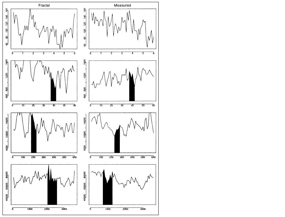
Figure 3: Synthesized traffic from a simple fractal model vs. Internet
traffic to which its mean, variance, and Hurst parameter (H) were
fitted, viewed over three orders of magnitude.
(from [willinger98where])
Let X =(Xt: t = 0, 1, ...) be a covariance stationary stochastic process; that is, a process with constant mean μ, constant variance σ, and autocorrelation function r(k)=E[(Xt-μ)(Xt+k-μ)]/E[(Xt-μ)2] that depends only on k. In particular, let's assume that r(k) ~ k-β L1(k), with 0 < β < 1 and L1 slowly varying at infinity. Let X(m) =(X(m)(k): t = 1, 2, ...) a new aggregate time series obtained by averaging the original time series X over non overlapping blocks of size m. The aggregate X(m) defines also a covariance stationary process with autocorrelation function r(m).
The process X is called (exactly second-order) self-similar with self-similarity (or Hurst) parameter H=1-β/2 if all the aggregate processes X(m) have the same autocorrelation function as X. In other words, X is exactly self similar if it is indistinguishable from its aggregate processes at least with respect to their second order properties.
The process X is called (asymptotically second-order) self-similar if, for large m, the corresponding aggregated time series have fixed correlation structure (determined by β).
To make the discussion more concrete and give an intuition about the meaning of this mathematical formulation, let us consider the example in Figs. 1 and 3. The time series in the first row represents the X process. The second row reports the aggregate process X(10), the third row shows X(100), and the last one reports X(500).
Notice that traditional stochastic processes have the property that, as m increases, the correlation function of the aggregated processes tends to 0. In other words, as m increases, the aggregated processes X(m) tend to a sequence of independent, identically distributed random variables (that is, covariance stationary white noise). On the contrary, the correlation function of (exactly or asymptotically) self-similar processes is nondegenerate. Also, remember that the concept of burstiness is in general bound to a non zero correlation between packet interarrival times.
In conclusion, two are the basic characteristics which distinguish self-similar processes from conventional stochastic processes:
Having discusses the basic concepts, we show in the next sections how LAN and WAN traffic has been characterized according to the presented models.
Several renewal traffic models have been proposed beside the Poisson one. Bernoulli processes can be seen as the discrete-time equivalent of Poisson models. If the interarrival times in a renewal process are of the so-called "phase type", we refer to phase-type renewal processes. Those processes can be modeled as the time to absorption in a continuous-time Markov chain [Wiki-Markov].
In a simple Markov traffic model, the interarrival times are exponentially distributed with different λi. A probability matrix is used in order to determine the rate parameter λi which should be used according to the system state i. In turn, the progress of the system state can be modeled through a Markov chain [Wiki-Markov]. The basic implication of this fact is the following: the conditional probability distribution of the system state in the future depends only on its current state (and not on its state in the past).
Markov-renewal models are more general: they allow the interarrival times to be arbitrarily distributed, and constrain the distribution to depend upon both the current state of the system and the interarrival interval. The state of the system is again modeled through a Markov chain.
Markov-modulated traffic models are characterized by an auxiliary Markov process which evolves in time and its current state controls the probability function of the underlying traffic mechanism. A particular subclass is the one of Markov-modulated Poisson processes, where the underlying model is Poisson.
In [lombardo98accurate] a Markov-based model for MPEG traffic is proposed. The authors show how the model captures both inter-group of frames and intra-group of frames correlation. Finally, they use the model to estimate the loss probability in an ATM multiplexer loaded by a MPEG video source and an aggragate of external traffic. [elsayed00superposition] introduces a methodology to approximately characterize the superposition process of N ≥ 2 arbitrary Markov renewal processes. In particular, the resulting process is modeled by a Markov renewal process with a state space growing with N. [robert95markov] introduces and validates a modulated Markov process which produces self-similarity on a finite time scale.
Autoregressive traffic models have been used in the modeling of video streaming traffic, were temporal locality between frames can be expressed by modeling a frame as a function of the previous ones. The reader is addressed to [alheraish] for a survey on autoregressive models in the context of videoconferencing systems.
The interested reader can find an analytical description of TES and some possible extensions to the basic model in [reichl97].
Figure 4: A pictorial representation giving an intuition of the self-similar behavior of Ethernet traffic: burstiness at different time scales is evident.
(from [#leland93selfsimilar])
The results can be summarized as follows:
Figure 5: Mean hourly connection arrival rates of several TCP sessions on a WAN scenario.
(from [#paxson95wide])
[paxson95wide] Vern Paxson and Sally Floyd, "Wide-area Traffic: The Failure of Poisson Modeling", IEEE/ACM Transactions on Networking, pp.226-244, June 1995. Available online at http://citeseer.ist.psu.edu/paxson95widearea.html
[jain86train] R. Jain and S. Routhier, "Packet Trains--Measurements and a New Model for Computer Network Traffic", IEEE Journal on Selected Areas in Communications, Vol. 4, Issue 6, pp. 986-995, September 1986 . Available online at http://www.cs.wustl.edu/~jain/papers/train.htm
[willinger98selfsimilarity] W. Willinger, V. Paxson, and M.S. Taqqu, "Self-similarity and Heavy Tails: Structural Modeling of Network Traffic". In A Practical Guide to Heavy Tails: Statistical Techniques and Applications, Adler, R., Feldman, R., and Taqqu, M.S., editors, Birkhauser, 1998. Available online at http://citeseer.ist.psu.edu/86873.html
[willinger98where] W. Willinger and V. Paxson, "Where Mathematics Meets the Internet", Notices of the AMS, Vol 45, No.8, P961-970, 1998. Available online at
[mandelbrot65] B. B. Mandelbrot, "Self-Similar Error Clusters in Communication Systems and the Concept of Conditional Stationarity", IEEE Transactions on Communications, Volume 13, Issue 1, pp 71- 90, March 1965
[leland91high] W. E. Leland and D. V. Wilson, "High time-resolution measurement and analysis of LAN traffic: Implications for LAN interconnection", Proc. of IEEE INFOCOM'91, pages 1360--1366, Bal Harbour, FL, USA, April 1991. Available online at http://citeseer.ist.psu.edu/leland91high.html
[leland93selfsimilar] W. E. Leland, M. Taqqu, W. Willinger and D. V. Wilson, "On the Self-Similar Nature of Ethernet Traffic," Proceedings of SIGCOM93, 1993, San Francisco, California, pp. 183-193. Available online at
[cao01nonstationarity] J. Cao, W. S. Cleveland, D. Lin, and D. X. Sun, "On the Nonstationarity of Internet Traffic," Proceedings ofACM SIGMETRICS, Volume 29, pp. 102-112, 2001. Available online at
[cao02internet] J. Cao, W. Cleveland, D. Lin, and D. Sun, "Internet traffic tends toward Poisson and independent as the load increases", in Nonlinear Estimation and Classification, D. Denison, M. Hansen, C. Holmes, B. Mallick, and B. Yu, Eds. New York, NY: Springer Verlag, Dec. 2002. Available online at http://citeseer.ist.psu.edu/cao02internet.html
[riedi00toward] R. H. Riedi and W. Willinger, "Towards an improved understanding of network traffic dynamics", in Self-similar Network Traffic and Performance Evaluation, Wiley, 2000, chapter 20, pp. 507-530. Available online at http://www.stat.rice.edu/~riedi/Publ/PDF/rw99.pdf
[elsayed00superposition] K.M. Elsayed and H.G. Perros, "The Superposition of Discrete-Time Markov Renewal Processes with an Application to Statistical Multiplexing of Bursty Traffic Sources," Technical Report TR 94-10, Dept of Computer Science, North Carolina State University, 1994. Available online at http://citeseer.ist.psu.edu/elsayed94superposition.html
[lombardo98accurate] A. Lombardo, G. Morabito, and G. Schembra, "An accurate and treatable Markov model of MPEG-video traffic", in Proceedings of IEEE INFOCOM '98, San Francisco, CA, March 1998. Available online at http://citeseer.ist.psu.edu/lombardo98accurate.html
[robert95markov] Robert, S. and Le Boudec, J.-Y. (1995a), "A Markov Modulated process for self-similar traffic.", Saarbr ucken, Schlo Dagstuhl, Germany, October 1995. Available online at http://citeseer.ist.psu.edu/robert95markov.html
[alheraish2004] A. Alheraish, "Autoregressive video conference models.", International Journal of Network Management, Vol. 14, Issue 5, 2004. Available online at http://portal.acm.org/citation.cfm?id=1024516
[reichl97] P. Reichl, M. Schuba, and S. Hoff, "How to Model Complex Periodic Traffic with TES.", in Proc. of 13th UKPEW Ilkley, West Yorkshire, July 1997, Available online at http://citeseer.ist.psu.edu/reichl97how.html
[rueda96survey] A. Rueda and W. Kinsner, "A Survey of Traffic Characterization Techniques in Telecommunication Networks", Canadian Conference on Electrical and Computer Engineering, 1996. Available online at http://citeseer.ist.psu.edu/rueda96survey.html
[frost94traffic] V. Frost and B. Melamed, "Traffic Modeling for Telecommunication Networks", IEEE Communications Magazine, 32(3), pp. 70-80, March, 1994. Available online at http://www.ittc.ku.edu/publications/documents/Frost1994_IEEE-Comm_mag-Traffic_modeling.pdf
Links:[Wiki-Poisson] Wikipedia - Poisson Distribution: http://en.wikipedia.org/wiki/Poisson_distribution
[Wiki-Self-similarity] Wikipedia - Self-similarity: http://en.wikipedia.org/wiki/Self-similar
[Wiki-Long-tail-traffic] Wikipedia - Long-tail traffic: http://en.wikipedia.org/wiki/Long-tail_traffic
[Wiki-Long-range-dep] Wikipedia - Long-range dependency: http://en.wikipedia.org/wiki/Long-range_dependency
[Wiki-Long-range-dep] Wikipedia - Pareto distribution: http://en.wikipedia.org/wiki/Pareto_distribution
[Wiki-Markov] Wikipedia - Markov Chain: http://en.wikipedia.org/wiki/Markov_chain