A Performance Model for a Thermally Adaptive Application Implemented in Reconfigurable HW
Abstract
A model is developed for estimating the performance of a thermally adaptive application. The goal of this model is to allow a user to estimate the performance impact of adjusting the thermal budget allotted an application for a given thermal condition. The model is developed by applying a multiple linear regression approach to experimentally obtained performance measurements. The thermal conditions used during the collection of performance measurements were a small subset of the large number of possible thermal conditions. The model is validated by comparing the performance predicted by the model against a set of performance measurements obtained using thermal conditions not included in the regression data set.
Table of Contents
1. Introduction
This section first motivates the general need for adaptive thermal management. Next a brief overview of the thermal management approach used in this case study is given. The goal of using a model to estimate application performance is then discussed. This section concludes with an outline summarizing the content and organization of this case study.
1.1 Motivation for Adaptive Thermal Management
Embedded applications can find themselves subjected to a wide range of thermal environments. This is especially true of mobile systems deployed in harsh thermal environments (e.g. space borne and military systems). High powered thermally aggressive applications that do not use some type of intelligent thermal management must either be over engineered with large fans and heat sinks, or must be operated significantly below their maximum computational capabilities.
Adaptive strategies for managing the thermals of an application can allow them to dynamically adjust their performance with respect to changes in environmental conditions. It was shown by Jones [Jones06fpt]that a thermally aggressive application achieved a 2.4 factor improvement in performance using and thermally adaptive frequency over the use of a thermally "safe" fixed frequency.
1.2 Thermal Management Approach
The adaptive thermal management approach used in this case study has three major components that impact application performance:
- Environment's ambient temperature
- Airflow over the device
- Thermal budget of the application
The first two components are defined by the thermal conditions in which the application is operating. The third (thermal budget) is set by the application user. The thermal budget defines the maximum allowed operating temperature of the application. As thermal conditions change the application performance adapts to stay within the allocated thermal budget. The details of this approach are described in section 3.2
1.3 Performance Model Goal
The goal of the performance model is to give the application user an estimation of what impact adjusting the application thermal budget will have on performance, for a given set of thermal conditions. There are situations where the user may not want to operate the application at the maximum thermal rating of the device. For example, the user may wish to limit application power consumption, or an embedded platform may contain several devices that have thermal budgets. In the second case, if there is an overall platform thermal budget, then the performance model can be used to estimate the performance trade-offs associated with the thermal budget setting of each device.
1.4 Outline
Section 2 presents related work in the field of thermal and power management. Section 3 describes the infrastructure used to implement the application under study. Section 4 describes the image correlation application under study. Section 5 presents the multiple linear regression approach used to develop the performance model. Section 6 first describes the experimentation setup used to collect performance measurements, and then gives the results of these measurements. Section 7 uses these results as input into the regression in order to compute model parameters, and then validates the model. Section 8 summarizes the key results of the case study
Back to Table of Contents
2. Related Work
This section gives an overview of related work in the field of thermal and power management. First a discussion of several mechanisms for measuring temperature is given. Next several techniques for dynamic thermal management (DTM) are introduced.
2.1 Measuring Temperature
A mandatory requirement of a thermal management mechanism is the ability to measure the temperature of the device housing the application. Lopez-Buedo [Lopez-Buedo00] provides a survey of several techniques for measuring temperature. These techniques focus predominately on silicon based devices, and include the use of thermal couples, thermal imaging cameras, and sense diodes embedded into the die.
A novel option presented for reconfigurable hardware devices, by Lopez-Buedo, is the configuration of ring oscillators in order to infer device temperature from changes in ring oscillator frequencies. This work with ring oscillators is later extended in [Lopez-Buedo04] using arrays of such oscillators to detect hot spots and thermal gradients in FPGAs.
This case study makes use of the embedded sense diode available on FPGAs manufactured by Xilinx Corporation to measure the junction temperature of the FPGA. Section 3.1 presents the details of how the sense diode is used.
2.2 Dynamic Thermal Management (DTM)
This section gives an overview of current work in the field of Dynamic Thermal Management (DTM) form industry and academia. Typically DTM includes the management of power as well the temperature of a device. First DTM applied to microprocessors is presented. This is followed by DTM applied to FPGA based systems.
2.2.1 DTM for Microprocessors
Microprocessors have been built that allow their voltage and frequency to be scaled to extend battery life of mobile computers. Companies that include Intel and AMD have extended this concept to manage heat dissipation on servers [Intel04dbs]. By introducing power management features, software running on the CPU can scale voltage and frequency to lower power usage before the device overheats. Such technology is critical for servers located in large data centers that house hundreds or thousands of computation nodes.
Low-power embedded processors like Xscale [Intel00x] have hooks that allow voltage and frequency scaling to manage power. Work presented by [Wirth04] makes use of these features to present a dynamic thermal management (DTM) system that scales processor frequency in response to temperature readings from an external thermal couple.
2.2.2 DTM for FPGAs
Shang performed power measurement experiments on the Xilinx Virtex-II FPGA to determine the distribution of dynamic power [Shang02]. For the applications analyzed it was found that as much as 22% of dynamic power was consumed by clock resources. Therefore managing the clock tree usage could result in significant power savings. The Virtex-II has entities called BUFGMUXs [Xilinx05v2], that can be used for shutting down part of the clock tree or switching to a low frequency during idle times [Choi03]. Meng showed a 25% power savings through low level simulation of a Wireless Channel Estimator application mapped to a Virtex-II, by disabling the clock for portions of the application not in use [Meng05].
Chow [Chow05] presents a dynamic voltage scaling mechanism that uses gate delay feedback to minimize the voltage supplied to internal FPGA logic, thereby reducing power consumption. The main idea of this work was to supply the minimum voltage to the FPGA needed by the critical path of an application to meet timing. It was shown that such an approach allowed scaling of the supply voltage with changes in temperature, since the gate delays of a circuit are dependent on device temperature.
The DTM approach used in this case study is based on work by Jones [Jones06fpt]. In this approach a thermal budget (i.e. maximum operating temperature) is associated with the application. A temperature feedback mechanism is used to adaptively scale the performance of the application. The goal of this approach is to maximum application performance for a specified thermal budget. Details of this approach are presented in section 3.2.
Back to Table of Contents
3. Platform Infrastructure Description
This section describes the two main components that make up the infrastructure used for this case study. First a brief description of the hardware platform is given. This is followed by a discussion of the DTM approach used.
3.1 Platform Hardware
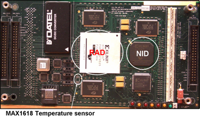
Figure 1: FPX Reconfigurable Hardware Platfrom
The FPX (Field-programmable Port eXtender) platform, shown in Figure 1, is used to implement the DTM mechanism and application used for this case study. This platform contains two FPGAs: (1) a small Xilinx Virtex FPGA called the Network Interface Device (NID) is configured with a static bitfile, and (2) a large Xilinx Virtex FPGA called the Reconfigurable Application Device (RAD) is reconfigured with bitfiles loaded dynamically over a network [Lockwood00]. New modular data processing functions are sent to the NID over the network within a bitfile that is used to reconfigure the RAD [Lockwood01]. The FPX uses an on-board Maxim temperature measurement device (MAX1618) to digitally compute the temperature of the RAD based on changes in the current produced by a thermal diode embedded in the RAD.
The application under study is implemented in the RAD, here after referred to as the Application FPGA. The controller portion of the DTM mechanism described in section 3.2 is implemented in the NID, here after referred to as the Management FPGA.
3.2 Thermally Adaptive Frequency Control
This section first gives a high level overview of the DTM approach used in this case study. Then some of the implementation details of the DTM approach are described.
3.2.1 Overview
The high level idea behind the DTM approach used in this case study is to modulate the duty cycle at which the application uses a slow clock and a fast (4x) clock. As the external thermal environment changes, the duty cycle automatically adjusts keeping the application temperature between an upper and lower temperature threshold. By selecting thresholds appropriately and switching quickly between modes, the application can maintain a target average temperature within tight bounds. The upper temperature threshold is the called the application thermal budget. The objective is to achieve maximum computational performance for a given thermal budget by adaptively adjusting the duty cycle as the thermal operating environment changes [Jones06fpt].
3.2.2 Implementation Details
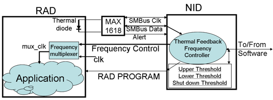
Figure 2: Thermal Management Architecture Mapped on the FPX Development Platform
The mapping of the thermally controlled adaptive frequency mechanism onto the FPX development platform is shown in Figure 2. This mechanism is made up of two components; 1) a dual frequency multiplexing circuit, and 2) a temperature driven frequency controller.
The select line (Frequency Control) of the frequency multiplexer determines if the base clock or 4x clock will drive the Application FPGA clock tree. Figure 3 shows the architecture of the frequency multiplexing circuit. The 4x clock generation part of this circuit uses a clock multiplier design supplied by the Xilinx application note number 174 [Xilinx00dll]. More elaborate techniques can and should be used to avoid clock glitches. For example a glitch free version of the 2:1 mux component can be implemented with the BUFGMUX component available for the Virtex-II [Xilinx05v2] and later generations of Xilinx FPGAs.
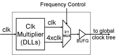
Figure 3: Frequency Multiplexer
The select line of the frequency multiplexing circuit is controlled by the temperature driven frequency controller, shown in Figure 2. This controller monitors the application temperature and implements a high/low temperature threshold control strategy. The Application FPGA operates using the 4x clock while the temperature remains below the upper threshold. Once the upper threshold is reached, the application circuit is given the base clock and allowed to cool down until the lower threshold is reached. At this point, the cycle repeats.
Back to Table of Contents
4. Application Description
This section first gives an overview of the characteristics of the image correlation application used in this case study. Next the services and performance metrics of the image correlation application are discussed. The section ends with a description of parameters and factors that impact application performance.
4.1 Image Correlation Application Overview
Image correlation has been shown in [Jones06fpt] to be a thermally aggressive application. This makes it a good candidate for modeling its performance with respect to thermal conditions. The implementation of the specific image correlation application used in this case study is the same as in [Jones06fpt].
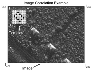
Figure 4: Image Correlation Algorithm Illustration
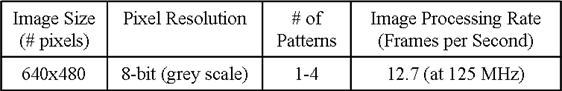
The image correlation algorithm scans an input image for 1 to 4 different patterns. Each pattern is called a template. Templates scan the image from left to right and from top to bottom. For each possible template position within the image a correlation score is computed. The correlation score is the sum of products of each template value with a corresponding image pixel value. Figure 4 helps to illustrate the image correlation algorithm implemented. Table 1 shows some of the characteristics of the image correlation application. Further details can be found in [Jones06fpt].
Table 1: Image Correlation Application Characteristics
4.2 Services and Performance Metrics
The main service provided by the image correlation application is to act as a filter for more complex image recognition software. The hardware implementation of the image correlation algorithm allows scores to be quickly computed, thereby allowing slower image recognition software to more quickly identify areas of interest within an image. More complex image recognition software can then analyze these selected areas in further detail.
The performance metric used for this application is the rate at which images can be processed, and is measured in frames per second (FPS). The value of 12.7 FPS given in Table 1 is the maximum rate at which this implementation of the algorithm can process images. In general the speed at which the application can process images is directly related to the frequency that the application can be run within the Application FPGA. This operating frequency is in turn dependent on environmental thermal conditions, as discussed in section 3.2
4.3 Parameters and Factors
This section presents the system and workload (operating condition) parameters that impact the performance of the image correlation application, and their ranges. Parameters that are identified for variation within the performance model are called factors. The ranges for which factors will be varied are specified.
4.3.1 System
The following system parameters impact the performance of the image correlation application:
- Thermal budget: This is the maximum temperature at which the image correlation application can run. This parameter is set by the application user. It is one of the factors used in the development of the performance model. For performance measurements this factor can take a value between 45 C and 65 C degrees.
- Minimum acceptable frame rate: This parameter indicates the minimum frame rate the application must be run in order to successfully identify moving objects. It is directly related to the minimum frequency used by the frequency multiplexing entity described in section 3.2.2. This parameter is fixed at 3 FPS, which equates to the application using a minimum frequency of 30 MHz.
4.3.2 Workload and Operating Conditions
The follow workload and operating conditions impact the performance of the image correlation application:
- Input image rate: The average rate and burstyness of incoming images impacts the performance of the application. It was shown in [Jones07vlsi] that for a given image input rate, images arriving evenly spaced in time give better performance than images arriving in large bursts. For this case study it is assumed that images are always available for the application to process. Thereby allowing the application to process images as quickly as thermal conditions will allow.
- Ambient temperature: This is the temperature of the environment in which the application is deployed. The lower the ambient temperature the longer the thermally adaptive frequency mechanism can run the application at its maximum frequency. This parameter is used as one of the factors in developing the performance model. For performance measurements this factor can have values ranging from 26C to 35C degrees. While ambient temperatures on earth can range from -40 C to 45 C, limitations of the experimentation environment dictate the use of a reduced range.
- Airflow over the FPGA: This is the airflow rate in Linear Feet per Minute (LFM), used to move heat away from the Application FPGA. For a stationary system airflow can range from 0 to about 2000 LFM. This parameter is used as one of the factors in developing the performance model. Due to limitations of the experimentation environment, a limited range of 0 to 500 LFM is used during performance measurements.
In summary thermal budget, ambient temperature, and airflow are the factors used in developing the performance model. During the development of the performance model these factors will be referred to as predictors.
Back to Table of Contents
5. Performance Model
This section describes the multiple linear regression approach used to develop a performance model for the image correlation application. First the assumptions made in the model are discussed. Next avoiding the problem of multicollinearity between ambient temperature and airflow is discussed. This section concludes with the construction of the performance model.
5.1 Assumptions
There are two major assumptions made by the performance model:
- All three predictors (thermal budget, ambient temperature, and airflow) are independent.
- All three predictors are linearly related to the performance of the image correlation application.
5.2 Avoiding Multicollinearity
It is particularly important to ensure the ambient temperature and airflow predictors are not correlated. If the performance measurement environment is not setup carefully, then these two predictors will become highly correlated. This would break the assumption of predictor independence given in section 5.1, and introduce the problem of multicollinerity (i.e. high correlation between predictors) [Jain91].
The experimentation setup used for this case study does not use an expensive environmental control chamber. Therefore if special precautions are not taken, then as airflow increases the ambient temperature within the case housing the application (see section 6.1) will fall until the ambient temperature of the room is reached. This issue is mitigated by placing an external heat source outside of the application housing, to warm air as it enters. The impact of the external heat source on ambient temperature is monitored by an electronic temperature probe located inside of the case. This gives verification that the housing ambient temperature is as specified.
5.3 Multiple Linear Regression
This section first introduces a method for performing a multiple linear regression. Next a procedure for analyzing the variation associated with the regression is presented.
5.3.1 Model
Multiple linear regression relates the response of one quantity (response variable) to k predictors. These predictors are assumed to be linearly related to the response variable (second assumption of section 5.1). The following is a summary of the multiple linear regression procedure given in [Jain91]. Multiple linear regression produces a model of the form:

Where
y is the response variable
b0 to bk are constant model parameters
x1 to xk are the model predictors
e is the error in measuring the response variable y
The model parameters are estimated by solving n simultaneous linear equations (Equation 1), each of these n equations represent the measured value of y at a specified value of the predictor variables.
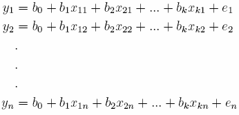
Equation 1: system of n linear equations for model construction
In vector form this group of linear equations can be represented as:
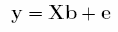
Equation 2: Vector form of multiple linear regression
where
y = the column vector of n observations
X = a matrix of predictor values with a size of n rows by k+1 columns
(Note the first column of this matrix is filled with 1's)
b = a column vector of the model parameters
e = a column vector of the errors associated with each collected observation
If it is assumed that the observation errors are random and uniformly distributed, then the sum of errors should be 0. Letting e = 0 gives the following when solving Equation 2 for b:
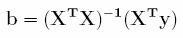
Equation 3: Solution for model parameters
Equation 3 gives the parameters needed to fully specify the model. For this case study:
k = 3 (i.e. there are 3 predictor variables)
b0 = the model offset constant
x1 = the Thermal budget predictor
b1 = the Thermal budget model parameter
x2 = the Ambient temperature predictor
b2 = the Ambient temperature model parameter
x3 = the Airflow predictor
b3 = the Airflow model parameter
Giving the following performance model to be used in this case study
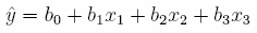
Where ŷ is the performance predicted by the model.
The next section presents a method to help evaluate if the prediction given by the model are significant compared to the error associated with the measured observations.
5.3.2 Analysis of Variation
Analysis of the variation of a model is an important part of determining if the results generated by the model are statistically significant. Table 2 reproduces a streamlined method to perform this analysis from [Jain91]. The basic purpose of analyzing the variation of the response variable is to determine the variation due to the regression model as compared to measurement errors.
Table 2: Multiple linear regression guide, reproduced from [Jain91]
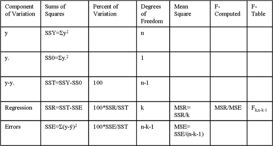
The column labeled "Percent of Variation" gives how much variation should be allocated to each of these two components. The notation y. refers to the mean of y. The F-Table value is the values obtained from an F-distribution at degrees of freedom (k, n-k-1). Where k is the degrees of freedom of the regression component, and n-k-1 is the degrees of freedom of the error component. If the F-Computed value is greater than the value found in the F-Table, then the variation due to the regression model is considered significant. One measure of the "goodness" of a regression is how much larger the regression variation is than the variation due to errors.
Another useful quantity that can be extracted from Table 2 is the standard deviation of the errors, and is given by:
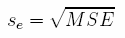
The standard deviation of errors can then be used to find the standard deviation of the computed model parameters and predictions of the response variable. These values can in turn be used to compute the confidence intervals of the model parameters and response variable. Using the general equation:

The t-value is obtained from a standard t-distribution table. Further details on performing the analysis of variation, and computing confidence intervals can be found in [Jain91].
Back to Table of Contents
6. Performance Measurement Experiments
This section first describes the experimentation environment used to collect performance measurements. This is followed by the presentation of collected performance measurements.
6.1 Experimental Setup
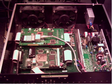
Figure 5: Experimentation Environment
The image correlation application is deployed on the Application FPGA of the FPX platform. The FPX was placed into a rackmount case, as shown in Figure 5. The case is equipped with 2 fans that each supplies approximately 250 Linear Feet per Minute (LFM) of air flow. The system has a removable case cover, not shown in Figure 5. Also not shown in Figure 5 is an additional cover and heat source used to produce ambient temperatures within the case that are greater than that of the laboratory.
The thermal budget is set by the user over a network interface to the Management FPGA. Airflow is controlled by the number of fans active; 0 LFM (no fans), 250 LFM (1 fan), 500 LFM (2 fans). Ambient temperatures larger than that of the laboratory are produced by warming the air entering the rackmount case with an external heat source.
6.2 Results
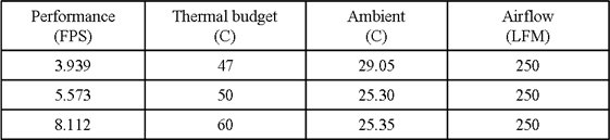
Table 3 and Table 4 present the results obtained from the performance measurement experiments. The results from Table 3 are used in section 7.1 for estimating model parameters. The results from Table 3 and Table 4 are used in section 7.2 to validate the model. Note the values in ( ) for Table 3 are the actual thermal budget and ambient temperature used for each experiment. Limitations of the setup prevent some combinations of predictor values to be used.
Table 3: Performance Measurements for Computing Model Parameters in Frames per second (FPS)
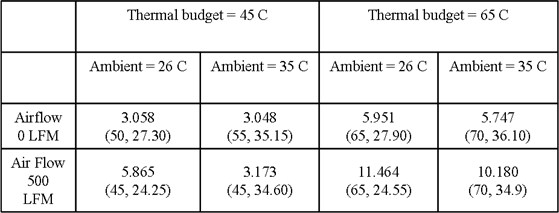
Table 4: Additional Performance Measurements for Model Validation
Back to Table of Contents
7. Analysis
This section first applies the performance measurements obtained in section 6.2 to the approach shown in section 5.3.1 for estimating model parameters. This section concludes with the model being validated against performance measurements obtain for predictor values not used for the estimation of model parameters.
7.1 Model Parameter Estimation
Using the procedure described in section 5.3, and the results form Table 3 the parameters for the performance model were found to be:
b0 = -4.168
b1 = .258
b2 = -.217
b3 = 7.490x10⁻³
where:
b0 = model offset constant
b1 = the model parameter for the thermal budget
b2 = the model parameter for the ambient temperature
b3 = the mode parameter for the airflow
Giving the following model for performance prediction:
yp = -4.168 + .258*x1 - .217*x2 + 7.49x10⁻³*x3
As a high level check, the sign value associated with each parameter agrees with intuition. It is expected that performance should increase when the thermal budget or airflow increases, and decrease when the ambient temperature increases. The following sections explore these results in more detail.
7.2 Analysis of Variation
As stated in 5.3.2 an analysis of variation for a model provides a method to determine if the variation due to the model is significant as compared to variation due to measurement errors. Table 5 provides the analysis of variation for the computed model.
Table 5: Analysis of variation of model
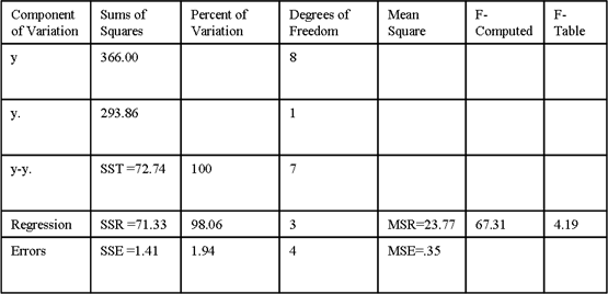
The results of this analysis show that 98% of the variation is due to the regression and only 2% is due to measurement errors. Since the F-Computed value is greater than the F-table value the variation due to the regression is significant. This gives evidence that the model fits the measured data well.
Taking the square root of the mean squared error (MSE) gives a standard deviation of .59 for measurement errors. Using this value the confidence intervals can be found for each of the model parameters. These intervals are:
b0 = (-7.92, -.41)
b1 = (.21, .31)
b2 = (-.32, -.12)
b3 = (5.63x10⁻³, 9.34x10⁻³)
None of the confidence intervals cross 0, therefore all model parameters are statistically significant. Note these intervals were computed at 90% confidence.
7.3 Model Validation
This section helps validate the model in two ways. First the assumption of predictor (factor) independence is evaluated using the correlation coefficient. Second, performance predictions from the model are compared against performance measurements obtained from conditions not used during model construction.
7.3.1 Factor Independence
The correlation coefficient, Rx1x2, between two predictors can be computed using Equation 4 [Jain91]. The correlation coefficient gives a measure of the amount of correlation between predictors, and has a value between -1 and 1. A value close to 0 indicates that the predictors show little correlation.
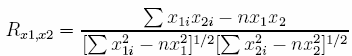
Equation 4: Correlation between two predictors
Letting:
x1 = Thermal budget
x2 = Ambient temperature
x3 = Airflow
gives the following values for the correlation coefficient between predictors:
Rx1x2 = .263
Rx1x3 = -.188
Rx2x3 = -.214
These values being close to 0 provides confidence that the predictors are independent. This also shows that the special precautions taken during experimental setup were effective in mitigating the ambient temperature dependency on airflow.
7.3.2 Validation Against Measured Performance
Computing the allocation of variation, section 7.2, is a good measure of how well the model fits the data used to compute model parameters. However it is important to also analysis how well the model matches performance measurements obtained from conditions not used to construct the model.
Table 6 gives the predicted response and measured response for 3 operating points not included in the construction of the model. From this table it can be see that the model gives a good estimate of application performance. The predictions are within about 10% of the measured values.
Table 6: Table 6: Predict response vs. measured response
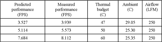
Further analysis of the predicted performance shows that, at 90% confidence, the model should predict results within 1.4 FPS. Therefore it appears that using a relatively small number of intelligently chosen observation points produces a reasonable model. If more observations were used the model should provide tighter bounds.
The main reason for using so small a number of observations was due to the expense in gathering observations. Each observation takes 30 minutes to an hour to collect. This case study gives evidence that reasonable results can be obtained by computing a model using predictor setting near the extremes of their range.
Back to Table of Contents
Summary
A multiple linear regression approach was used to create a performance prediction model for a thermally adaptive image correlation application. A small subset of observations from the large number of possible thermal conditions was used to construct the model. A major motivation for using a small subset of observations was the expense associated with collecting each observation (30 minutes - 1 hour).
The analysis and validation of the model gave evidence that the two major assumptions made by the model were reasonable. First the assumption of independence between predictors was evaluated by computing the correlation coefficient between predictors. The results of these computations indicated a relatively small correlation among predictors. Second the assumption of linearity between the predictors and system response was supported by the large amount of variation due to the model (98%) relative to errors (2%).
The final results of this case study showed that reasonable predictions could be obtained by using a small number of intelligently chosen observation points. These points were selected by using values near the minimum and maximum value for each predictor. Since this model uses a small number of predictors, 3, it was feasible to collect measurements for all combinations of min/max values (total of 23 = 8 measurements). During the validation of this model it was shown that predictions were within about 10% of measured values, for observations not used during model construction.
Back to Table of Contents
References
-
[Jones06fpt] Phillip H. Jones and Young H. Cho and John W. Lockwood, "An Adaptive Frequency Control Method using Thermal Feedback for Reconfigurable Hardware Applications," To appear in Proceedings of the IEEE International Conference on Field Programmable Technology (FPT '06),
http://liquid.arl.wustl.edu/publications/FPT_Adapt_Freq.pdf
Provides Details of the Thermally Adaptive Frequency Mechanism used in this Case Study.
-
[Jain91] Raj Jain, "The Art of Computer Systems Performance Analysis," pages 244-254,
http://www.cse.wustl.edu/~jain/books/perfbook.htm
Chapter 15 Provides an Overview of Multiple Linear Regression.
-
[Lopez-Buedo00] Sergio Lopez-Buedo, Javier Garrido, Eduardo Boemo, "Thermal Testing on Reconfigurable Computers," IEEE Design and Test of Computers, vol 17,
http://www.ii.uam.es/~ivan/dt00-test.pdf
Provides a Survey of Methods for Measuring Device Temperature.
-
[Lopez-Buedo04] Sergio Lopez-Buedo and Eduardo I. Boemo, "Making visible the thermal behaviour of embedded microprocessors on FPGAs: a progress report," In Proceedings of the International Symposium on Field-programmable Gate Arrays (FPGA '04),
http://www.ii.uam.es/~ivan/02004-acmfpga04-thermal-up.pdf
Provides a Case Study of using Ring Oscillators to Measure FPGA Temperature.
-
[Lockwood00] John W. Lockwood and Jon S. Turner and David E. Taylor, "Field Programmable Port Extender (FPX) for Distributed Routing and Queuing," In Proceedings of International Symposium on Field-Programmable Gate Arrays (FPGA '00),
http://ipoint.vlsi.uiuc.edu/publications/fpga2000_fpx.pdf
Provides details of the FPX Platform
-
[Lockwood01] John W. Lockwood and Naji Naufel and Jon S. Turner and David E. Taylor, "Reprogrammable Network Packet Processing on the Field Programmable Port Extender (FPX)," In Proceedings of International Symposium on Field-Programmable Gate Arrays (FPGA '01),
Description of the FPX being used to send Network Processing Hardware Modules over a Network .
-
[Jones07vlsi] Phillip H. Jones and Young H. Cho and John W. Lockwood, "Dynamically Optimizing FPGA Applications by Monitoring Temperature and Workloads," To appear in Proceedings of the IEEE International Conference on VLSI Design (VLSI Design '07),
http://liquid.arl.wustl.edu/publications/VLSI_Therm_Load_adapt.pdf
Provides a Study of the Impact of Input Burstyness on Device Thermals and Latency.
-
[Intel04dbs] Intel Corporation, "Addressing Power and Thermal Challenges in the Datacenter," White Paper,
http://www.intel.com/products/services/intelsolutionservices/success/techdocs/wp/thermal.pdf
Introduces the Demand Based Switching (DBS) Technology used by Intel Servers.
-
[Intel00x] Intel Corporation, "Intel 80200 Processor based on Intel XScale Microarchitecture Developer's Manual,", Chapter 8
http://systems.cs.colorado.edu/Documentation/IntelDataSheets/80200developersmanual.pdf
Provides Detail of Xscale Software Programmable Internal Clock Frequency.
-
[Wirth04] Eric Wirth, "Thermal Management in Embedded Systems ," Thesis,
http://www.cs.virginia.edu/~skadron/Papers/wirth_thesis.pdf
Gives Details on how to Implement Dynamic Thermal Management (DTM) on the Xscale Processor.
-
[Shang02] Li Shang and Alireza S. Kaviani and Kusuma Bathala, "Dynamic power consumption in Virtex-II FPGA family," In Proceedings of International Symposium on Field-Programmable Gate Arrays (FPGA '02),
http://www.ece.queensu.ca/hpages/faculty/shang/papers/fpga02.pdf
Provides a Case Study of the Distribution of Power on an FPGA.
-
[Xilinx05v2] Xilinx Corporation, "Virtex-II Platform FPGA User Guide," page 70,
http://www.xilinx.com/bvdocs/userguides/ug002.pdf
Introduces the BUFGMUX Component for Multiplexing between Clocks.
-
[Choi03] Seonil Choi and Ronald Scrofano and Viktor K. Prasanna and Ju-Wook Jang, "Energy-efficient signal processing using FPGAs," In Proceedings of International Symposium on Field-Programmable Gate Arrays (FPGA '03),
http://ceng.usc.edu/~prasanna/papers/choifpga03.pdf
Calls out the use of the Virtex-II BUFGMUX as a Technique for Energy-Efficient Design.
-
[Meng05] Y. Meng and W. Gong and R. Kastner and T. Sherwood, "Algorithm/Architecture Co-exploration for Designing Energy Efficient Wireless Channel Estimator," Journal of Low Power Electronics, vol 1,
http://www.cs.ucsb.edu/~sherwood/pubs/JOLPE-channelest.pdf
Case Study of Power Savings obtained from Disabling unused Portions of a Clock Tree.
-
[Chow05] C. T. Chow and L. S. M. Tsui and P. H. W. Leong and W. Luk and S. J. E. Wilton, "Dynamic Voltage Scaling for Commercial FPGAs," In Proceedings of the IEEE International Conference on Field Programmable Technology (FPT '05),
http://pubs.doc.ic.ac.uk/dvs/dvs.pdf
Uses Critical Path Delay Feedback to Scale FPGA Frequency.
-
[Xilinx00dll] Xilinx Corporation, "Using Delay-Locked Loops in Spartan-II FPGAs," Xilinx Application Note 174,,
http://www.xilinx.com/bvdocs/appnotes/xapp174.pdf
Describes how to use Delay Lock Loops (DLLs) to build Clock Multipliers.
Back to Table of Contents
List of Acronyms
| DTM |
Dynamic Thermal Management |
| FPGA |
Field Programmable Gate Array |
| FPS |
Frames Per Second |
| FPX |
Field-programmable Port eXtender |
| LFM |
Linear Feet per Minute |
| NID |
Network Interface Device |
| RAD |
Reconfigurable Application Device |
Back to Table of Contents
This report is available on-line at
http://www.cse.wustl.edu/~jain/cse567-06/thermal.htm
List of other reports in this series
Back to Raj Jain's home page