ESE297 - Intro to Undergraduate Research

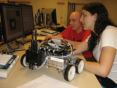
The Robotics Sensing Training Course was created for students who wish to do Undergraduate Research projects in Robotic Sensing under Professor Nehorai, the ESE Department Chair. This course is offered as ESE497B for 2 credits and is typically offered in the spring and summer. Students will learn how to implement sensor array signal processing algorithms on the LabVIEW for Robotics Starter Kit robots shown above using both Matlab and LabVIEW. Students can then apply this knowledge to individual research projects in Robotic Sensing in subsequent semesters.

Logistics

• Meeting Time: Monday, Wednesday 9-12 starting May 24 through July 14 in Bryan 316
• Holidays: 5/31, 7/5
• Supervisor: Phani, Pato, Ed
• Faculty Supervisor: Arye Nehorai
• Expectations: Each student needs to work 10 hours/week in order to earn the 2 credits for ESE497. In the summer, the expectation is 20 hours/week. That is, students who earn an A will spend many unsupervised hours outside of the class meeting times. In Part 1 of the class, homework will be assigned and is due during the next class meeting. The project (Part2 below) should be completed by the end of the semester.

Course Details

• Part1: Case Study - Study acoustic source localization using Microphone array (see Lecture Notes below)
  • Background and Theory
  • Data Acquisition Basics
  • Introduction to Digital Signal Processing Tools
• Part2: Implement algorithm with microphone array and USB Data Acquistion
• Part3: Implement algorithm with sbRIO robots
• Part4: Put the sbRIO robots in motion

Lecture Notes

• Topic 1: Acoustic Source Location Background and Theory
  • Additional references:
    • Joshua York, Acoustic Source Localization, ESE497, Fall 2008
    • Raphael Schwartz and Zachary Knudsen, Robotic Microphone Sensing: Data Processing Architectures for Real-Time, Acoustic Source Position Estimation, ESE497, Fall 2009
  • Task 1: Read the material that we discussed in our meeting today and the additional references listed above.
  • Task 2: Using the bottom diagram on MicSourceLocatorSolution -> My Computer -> MicSourceLocator-Array.vi -> Simulator.vi, derive the equations for the source location, i.e., the intersection of the 2 lines. Verify that the formula on slide 10 is correct for that special case where y1 = y2 = 0 and Rotation1 and Rotion2 = 0.
• Topic 2: Data Acquisition Basics
  • LabVIEW Tutorial
    • Conditionally append values to an array in a loop
    • How to Create and Array on the Front Panel
    • Additional LabVIEW tutorials
    • Task 3 - Finish Exercises
  • Data Acquisition Basics
    • Task 4 - Finish exercise
    • Task 5 (due 2/10/2010)
      • Connect wires from A00 and AO1 to AI0+ and AI1+ (remove wire from Banana A to AI0+). Make sure that the Prototyping Power is on. Modify your vi from Task 4 to collect samples from both AI0 and AI1. Then open DelayedChirp2DAC.vi and run this vi. You shouldn't modifiy DelayedChirp2Dac.vi. Run your modified Task 4 vi and zoom in in the time and frequency domain to examine the waveforms in detail. Describe in detail what you see. Measure the difference in time between both channels. Hint: Start and stop your Data Acquisition vi until the entire signal is in the middle of the buffer.
      • Plot the Cross Correlation of the 2 channels and see if the peak is shifted from the middle, the number of samples you measured from the previous step.
        • Hints:
          • Functions -> Express -> Conv & Corr -> Cross Correlation
          • This function requires that you extract the 2 channels from the DDT. To do this, use Functions -> Express -> Sig Manip -> From DDT -> Single Waveform -> Channel 0 and then again for Channel 1. Connect the outputs of these to the X and Y inputs.
          • Before you plot the Cross Correlation, extract the 1D array of scalars using the From DDT so that the X-Axis is in samples.
          • Look at the help on the Cross Correlation for details.
      • Plot the Spectrogram of Channel 0.
        • Hint: There is a good Spectrogram example that ships with LabVIEW. Go to Help -> Find Examples... and search for Spectrogram -> STFT Spectrogram Demo.vi. You can copy from this example and paste it into your code.
• Topic 3: Filters Basics
  • Tutorial
    • Task 6- Finish exercise from tutorial.
      • Solution
    • Task 7- Use the Signal Processing Palette in LabVIEW to generate 2 sinusoid waveforms (Signal Processing -> Waveform Generation -> Sine Waveform) with two different frequencies. Add these together and filter this signal twice to obtain the two sinusoid signals corresponding to two frequencies of the input signals. Then, add (as in addition) Gaussian White Noise to this signal (Signal Processing -> Waveform Generation -> Gaussian White noise). Plot the spectrum (Express-> Signal Analysis -> Spectral) of this signal and identify the frequencies corresponding to signal and noise. Use an appropriate filter (Express -> Signal Analysis -> Filter) to extract the original 2 signals. Repeat with various filters and with increasing noise power. What is the relationship between the Standard Deviation of the WGN and the amplitude of the noise (Express -> Signal Analysis -> Histogram might help)? Note: If your graph X-axis is in absolute time instead of seconds, right click on the graph and select Properties -> Display Format -> X-Axis and set it to SI units.