Difference between revisions of "The Methods"
ChuckHolmes (talk | contribs) |
ChuckHolmes (talk | contribs) |
||
| (5 intermediate revisions by the same user not shown) | |||
| Line 7: | Line 7: | ||
==Step 2: Initialization== | ==Step 2: Initialization== | ||
| − | From | + | From a MATLAB terminal, the user calls a MATLAB script. For this particular experiment, the script was called "Therm3d_sdk_cdh.m". |
For the most part, this first step involves initializing and calibrating the various devices associated with the script. At most parts of this first step, the script will prompt the user to press any key when the initializing action is complete. | For the most part, this first step involves initializing and calibrating the various devices associated with the script. At most parts of this first step, the script will prompt the user to press any key when the initializing action is complete. | ||
| Line 29: | Line 29: | ||
====Callibrating the Thermocouples==== | ====Callibrating the Thermocouples==== | ||
| − | The script will ask the user to place the thermocouples under the ThermoHaake thermistor and verify that they are there with a key press. For each thermocouple, a temperature measurement will be made. Then the thermocouple measurement system will be modified to match the ThermoHaake thermistor. This is done by observing the equation | + | The script will ask the user to place all the thermocouples under the ThermoHaake thermistor and verify that they are there with a key press. For each thermocouple, a temperature measurement will be made. Then the thermocouple measurement system will be modified to match the ThermoHaake thermistor. This is done by observing the equation |
<math>y=mx+b</math> | <math>y=mx+b</math> | ||
| Line 68: | Line 68: | ||
===Data Acquisition=== | ===Data Acquisition=== | ||
| − | If an equilibrium is reached, then images are taken at different slices of the tissue. If an equilibrium is not reach in a certain time, determined by a header file parameter, then imaging occurs as though equilibrium had been reached. These images are then saved in the "ult" | + | [[File:Video.gif|thumb|right|''Figure 2 - Slice 15 at increasing temperatures]] |
| + | If an equilibrium is reached, then images are taken at different slices of the tissue. If an equilibrium is not reach in a certain time, determined by a header file parameter, then imaging occurs as though equilibrium had been reached. These images are then saved in the "ult" directory in the experiment directory. The images are saved with the name "(experiment ID)_(temperature)_(slice number)". | ||
After the images are taken, the archived matrices are saved in a mat-file named "(experiment ID)exp.mat". | After the images are taken, the archived matrices are saved in a mat-file named "(experiment ID)exp.mat". | ||
| + | |||
| + | After every temperature has been visited, the "ult" directory will contain the pictures from every slice for every temperature. Figure 2 shows slice 15 at increases temperatures. Notice how it appears to rise. This is because increased temperature in the water allows for faster propagation of the ultrasound. | ||
Latest revision as of 06:52, 13 May 2011
This page will go over the procedure of the experiment. This page also functions as a user's manual for running an experiment.
Contents
Step 1: Setup
To start, the tissue must be cut to fit in the experimental housing. This is best done with a pair of scissors. After it is cut, it is placed in the housing and the housing is placed in the insulated container.
A series of filters and a degassing vacuum are used to deionize and degas some water. The water is used to fill the container. On the underside of the ThermoHaake is a float. The proper amount of water to use in filling the container is enough water to lift the float. Without lifting the float, the ThermoHaake will not function.
Step 2: Initialization
From a MATLAB terminal, the user calls a MATLAB script. For this particular experiment, the script was called "Therm3d_sdk_cdh.m".
For the most part, this first step involves initializing and calibrating the various devices associated with the script. At most parts of this first step, the script will prompt the user to press any key when the initializing action is complete.
Windaq and the DATAQ: Part 1
The script will start up the Windaq software.
The script will ask the user to press any key when Windaq is running. When a key is pressed, the script will proceed.
Header File
Associated with each experiment is a header file (.HDR), which contains all the experiment's parameter information. Examples of parameters contained in the header file include
- Experiment name
- Temperature Set (the temperature that will be observed over the course of the experiment)
- Numbers of Channels to be used for temperature measurement
The script parses the header file and sets script variables to be equal to header file parameters.
ThermoHaake
The ThermoHaake pump speed is set to an appropriate value (for now it is a hard-coded value of 50). Then the water is circulated with no heating. This is accomplished by setting the target temperature (or temperature to be heated to) to 10 degrees Celsius and pumping the water. The water is pumped to ensure that the there is little to no temperature gradient in the water for the rest of the initialization process.
Windaq and DATAQ: Part 2
Callibrating the Thermocouples
The script will ask the user to place all the thermocouples under the ThermoHaake thermistor and verify that they are there with a key press. For each thermocouple, a temperature measurement will be made. Then the thermocouple measurement system will be modified to match the ThermoHaake thermistor. This is done by observing the equation
<math>y=mx+b</math>
where y is the temperature output of the system (or the measurement), x is the temperature input (or the actual measurement of the thermocouple), m is the slope which is a parameter of the thermocouple, and b is the offset which is determined by this part of the experiment.
The slopes are predetermined and saved as mat-file (in this case as TCSlopes.mat). The script loads the mat-file and passes the values into further calculations.
The offset is determined by the shifting of the previous equation to be
<math>b=y-mx</math>.
We know x and m. If use the ThermoHaake thermistor measurement, which we treat as the actual temperature of the water, as our y value, then we can solve for b.
Thermocouple Placement
The script then asks the user to place the thermocouples in their experimental positions. One thermocouple is placed directly below the the ThemoHaake. Another thermocouple is placed on the opposite end of the insulated container. The remaining four thermocouples (6 in total are used) are placed in the tissue.
The user will be prompted to verify when this is done.
The Newport and the Ultrasound Transducer
The script will ask the user if the Newport turned on. When it is turned on and a key has been pressed to verify that it is on, the script will proceed.
The Newport will then move the transducer from one end of the tissue to the other. All this time, the ultrasound transducer is taking images of the tissue. The user can use this "scan" as an opportunity to verify that the transducer is placed right, the thermocouples are in the view of the image, etc.
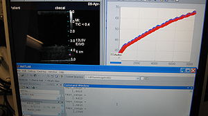
For a view of the Terason user interface, see Figure 1. The upper left corner shows the Terason's ultrasound image viewer.
Step 3: Heating the Water Bath and Data Acquisition
Heating the Water
The ThermoHaake will begin an iteration that heats the water bath to temperature values in the temperature set parameter. For each temperature in the set, the ThermoHaake will heat and circulate the water bath until the temperature is reached. For this part of the process, the ThermoHaake will set the target temperature to be half a degree larger than the true target temperature.

As the temperature of the water approaches target temperature, the system will repeat three steps. First, the system will acquire the temperature measurements from all the thermocouples and the ThermoHaake thermistor. Then the MATLAB script will plot these values against the time they were observed. An example of a plot can be seen in Figure 1 in the upper right corner. The red data represents measurements made in tissue and blue data represents measurements made in the water. Finally, the script will archive the temperature measurements by concatenating the values to a matrix. At the end of the experiment, these matrices will be saved.
This sequence of events repeats until a the target temperature is reached. When the true target temperature is reached, the ThermoHaake target temperature will be set to 10 degrees Celsius so that while circulation can continue in the water, heating cannot occur. This is to facilitate the tissue reaching a temperature equilibrium. At this point, the script enters a sub-iteration in which temperature measurement, plotting, and archiving still occurs as before. This will continue until a temperature equilibrium is reached.
Equilibrium is reached when the difference between the greatest thermocouple measurement and the the least thermocouple measurement is less than a equilibrium constant, which has a value determined by a header file parameter.
Data Acquisition
If an equilibrium is reached, then images are taken at different slices of the tissue. If an equilibrium is not reach in a certain time, determined by a header file parameter, then imaging occurs as though equilibrium had been reached. These images are then saved in the "ult" directory in the experiment directory. The images are saved with the name "(experiment ID)_(temperature)_(slice number)".
After the images are taken, the archived matrices are saved in a mat-file named "(experiment ID)exp.mat".
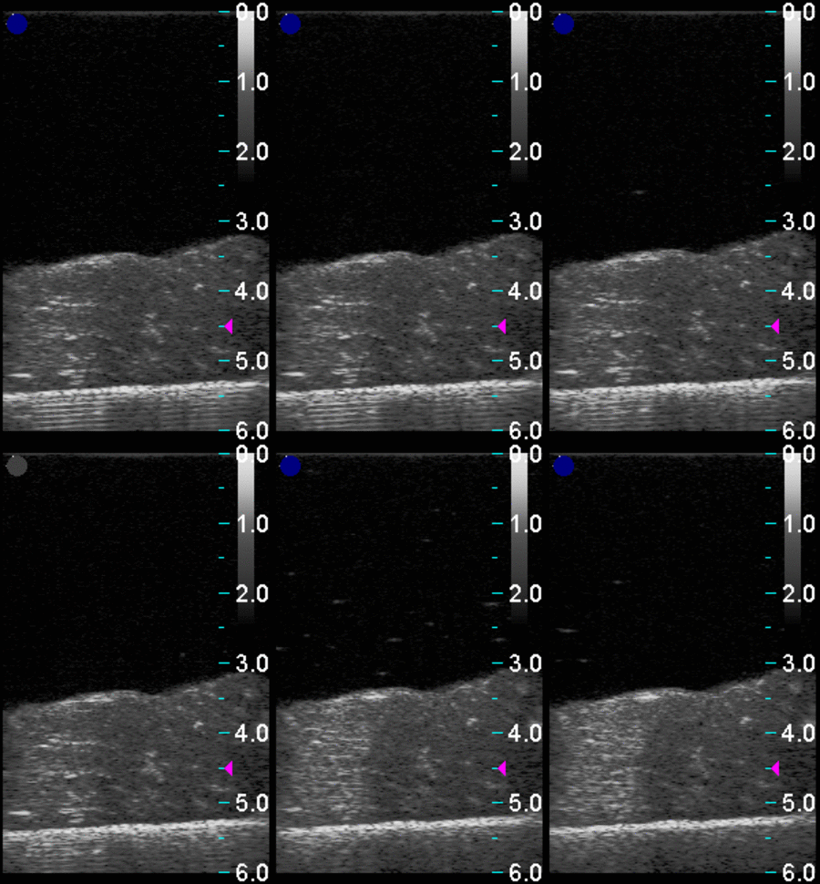
After every temperature has been visited, the "ult" directory will contain the pictures from every slice for every temperature. Figure 2 shows slice 15 at increases temperatures. Notice how it appears to rise. This is because increased temperature in the water allows for faster propagation of the ultrasound.
