Response spectrum analysis is intended to provide an inexpensive approach to estimating the peak response of a model (usually a model of a structure) subjected to “base motion”: the simultaneous motion of all nodes fixed with boundary conditions. The approach assumes that the system's response is linear, so it can be analyzed in the frequency domain using its lowest eigenmodes——and eigenfrequencies —extracted in a previous eigenfrequency step. The method is typically used to estimate the response of a building or of a piping system in a building to an earthquake. The method is not appropriate if the excitation is so severe that nonlinear effects in the system are important. In such a case the time history of the base excitation must be known and used with a dynamic analysis step to obtain the system's response.

Even for a linear system the response spectrum method provides only estimates of the peak response. If more precise values are required, a modal dynamic analysis step can be used to integrate the system through time and, thus, develop its response to the given base excitation.

In response spectrum analysis the estimates of peak values are obtained by combining the peak responses of the participating modes corresponding to user-specified spectra definitions. Several approximations are introduced by response spectrum analysis. The conversion from a time history of excitation into an equivalent frequency domain spectrum is based on the behavior of a single degree of freedom system. Different spectra are often applied in different excitation directions. Once the spectra are known, the peak modal responses can be calculated. The manner in which these peak modal responses are combined to estimate the peak physical response, together with the manner in which multidirectional excitations are combined, introduces approximations. Since no one method gives good approximations for all cases, several methods are offered. These methods are discussed in the Regulatory Guide 1.92 (1976) of the U.S. Nuclear Regulatory Commission, in the papers by Anagnastopoulos (1981), Der Kiureghian (1981), and Smeby (1984) and in the book by A. K. Gupta (1990). The choice of the summation rules depends on the particular case and is a matter of the user's judgment.

Since response spectrum analysis is commonly used as a basic design tool, spectra are defined in many design codes for such applications as seismic analysis of buildings. In such cases the user works from the given spectra. In other cases the time history of a known base excitation must first be converted into a response spectrum by considering the response of a single degree of freedom system excited by the known base motion. For this purpose the single degree of freedom system is characterized by its undamped natural frequency, , and the fraction of critical damping present in the system, . The equation of motion of the system is integrated through time to find peak values of relative displacement, relative velocity, and absolute acceleration. The integration described in “Modal dynamic analysis,” Section 2.5.5, can be used for this purpose, since it is exact when the base motion record varies linearly with time. Thus, the maximum values of displacement, velocity, and acceleration are found for the linear, one degree of freedom system. This process is repeated for all frequency and damping values in the range of interest to construct displacement, velocity, and acceleration spectra, , and . A FORTRAN program to build spectra in this way from an acceleration record is given in “Analysis of a cantilever subject to earthquake motion,” Section 1.4.13 of the ABAQUS Benchmarks Manual (file cantilever_spectradata.f.)

If there is no damping, the relationship between , , and is given by

In ABAQUS/Standard it is assumed that the damping is always small, so these relationships are used whenever a conversion is needed.

A response spectrum is defined by giving a table of values of at increasing values of frequency, , for increasing values of damping, . Linear interpolation on a logarithmic scale is used to compute the response for any required frequency and damping factor. Any number of spectra can be defined.

The response spectrum procedure allows up to three spectra, which we denote by , , to be applied to the model in orthogonal physical directions defined by their direction cosines, . These spectra can come from different excitations (with a certain level of correlation between them), or they can be components of a single base excitation acting in an arbitrary direction.

When modal methods are used to define a model's response, the value of any physical variable is defined from the amplitudes of the modal responses (the “generalized coordinates”), . The first stage in the response spectrum procedure is to estimate the peak values of these modal responses. For mode and spectrum this is

where is a user-defined scaling parameter, is the th displacement spectrum, is the th direction cosine for the th spectrum, and is the participation factor for mode in direction (see “Variables associated with the natural modes of a model,” Section 2.5.2, for the definition of ). Similar expressions for and are obtained by using velocity or acceleration spectra in the above formula.

We now have estimates of the peak responses of the “generalized coordinates”—the amplitudes of the responses of the natural modes of the system for excitation in each direction. If the input spectra in the different directions are components of a single base excitation acting in an arbitrary direction, for each mode we can combine these peak responses into a single value by specifying algebraic summation of the values for the different spatial directions:

In this case the modal combinations discussed below still apply, but the subscript is no longer relevant and should be ignored.

Let us denote by the peak response of some physical variable (a component of displacement, stress, section force, reaction force, etc.) caused by motion in the natural mode excited by the response spectrum in excitation direction at frequency and with damping . Denote the component of the eigenvector associated with by . Then

and

We need to combine these estimates of the peak physical responses in the individual modes into estimates of the total peak response of the particular physical variable to the given spectrum, . Since the peak responses in the different modes will not in general occur at the same time, this combination is only an estimate, so several formulæ are offered, as follows:

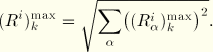
Summation of the absolute values of the modal peak responses estimates

This provides the most conservative estimate of the peak response, since it assumes that all modes provide peak response in phase at the same time.

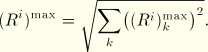
Square root of the summation of the squares (SRSS) estimates

This summation usually provides a reasonable estimate if the natural frequencies of the modes are well separated.

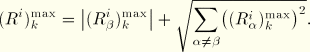
The Naval Research Laboratory method distinguishes the mode, , in which the physical variable has its maximum response, and adds the square root of the sum of squares of the peak responses in all other modes to the absolute value of the peak response of that mode. This gives the estimate

Again, the modes must be reasonably well-spaced in the frequency domain to obtain an accurate estimate with this method.

A variety of methods are available that aim to improve the estimation for structures with closely spaced frequencies. ABAQUS/Standard provides two of them: the Ten Percent method recommended by Regulatory Guide 1.92 (1976) of the U.S. Nuclear Regulatory Commission and the complete quadratic combination method, which was first introduced by Der Kiureghian (1981) and developed by Smeby and Der Kiureghian (1984). Both methods reduce to the SRSS method if the modes are well separated with no coupling among them.

The Ten Percent method described in Regulatory Guide 1.92 modifies the SRSS method by adding a contribution from all pairs of modes and whose frequencies are within 10% of each other, giving the estimate

The frequencies of modes and are considered to be within 10% whenever

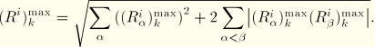
The complete quadratic combination method (CQC) combines the modal response with the formula

where are cross-correlation coefficients between modes and , which depend on the ratio of frequencies and modal damping between the two modes: where If double eigenvalues occur with the same damping coefficient, their correlation coefficient will be . If modes are well-spaced, their cross-correlation coefficient will be small () and the method will give the same results as the SRSS method. This method is usually recommended for asymmetrical building systems, since, in such cases, other methods can underestimate the response in the direction of motion and overestimate the response in the transverse direction (see “Response spectra of a three-dimensional frame building,” Section 2.2.3 of the ABAQUS Example Problems Manual).

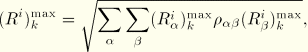
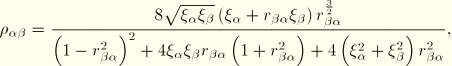
For the case of different base excitations acting along orthogonal directions, we still need to sum over the directions indicated by the subscript . Regulatory Guide 1.92 specifies that this directional summation be based on the square root of the sum of the squares summation rule:

This rule is appropriate when the base motions in different directions are statistically independent (uncorrelated)—when they are acting along “principal directions.” The existence of a set of directions along which the ground motions can be considered uncorrelated is discussed by Penzien and Watabe (1975). Such considerations are especially important when the CQC modal combination method is used. In the ABAQUS implementation of the CQC method it is assumed that the horizontal components act along the principal directions and are of equal intensity. For details on the CQC method applied to more general cases, see Smeby and Der Kiureghian (1984).